Data quality adjustment

Background and purpose

Objective of the module

The Data Quality Adjustment module addresses two common limitations of routine health facility data: extreme values resulting from reporting or data entry errors (outliers) and gaps arising from incomplete reporting (missing data). Rather than excluding affected observations, the module replaces these values with statistically derived estimates informed by each facility’s historical reporting patterns.

The adjustment process applies time-series smoothing methods that draw on observed trends and seasonality within facility-level data. Rolling averages and facility-specific historical profiles are used to correct anomalous values while preserving underlying service delivery patterns.

To support transparency and analytical flexibility, the module generates four parallel datasets: unadjusted data, data with outlier corrections only, data with missing values imputed only, and data with both adjustments applied. This allows users to assess the sensitivity of results to different data quality assumptions and select the dataset most appropriate for their analytical purpose.

Analytical rationale

Routine health management information system (HMIS) data frequently contain reporting errors and gaps that can distort observed trends and obscure underlying patterns in service delivery. Extreme values may create artificial spikes in service volumes, while incomplete reporting can result in apparent declines that reflect data quality issues rather than true changes in service provision. These limitations are particularly consequential when HMIS data are used for performance tracking, comparison across geographic units, or trend analysis.

By systematically addressing outliers and missing data prior to analysis, this module improves the consistency and interpretability of HMIS data. This helps ensure that subsequent analytical outputs are based on observed service delivery patterns rather than artifacts introduced by reporting variability or data quality constraints.

Key points

Component	Details
Inputs	Raw HMIS data (hmis_ISO3.csv) Outlier flags from Module 1 (M1_output_outliers.csv) Completeness flags from Module 1 (M1_output_completeness.csv)
Outputs	Facility-level adjusted data (M2_adjusted_data.csv) Subnational aggregated data (M2_adjusted_data_admin_area.csv) National aggregated data (M2_adjusted_data_national.csv) Exclusion metadata (M2_low_volume_exclusions.csv)
Purpose	Replace outlier values and fill missing data using facility-specific historical patterns; produces four adjustment scenarios (none, outliers only, completeness only, both)

---

Analytical workflow

Overview of analytical steps

The module applies a standardized, multi-step process to adjust routine health facility data while preserving underlying service delivery patterns:

Step 1: Load and prepare data The module integrates three inputs: reported facility-level service volumes (hmis_ISO3.csv), outlier flags identifying anomalous values (M1_output_outliers.csv from Module 1), and completeness flags indicating months with incomplete reporting (M1_output_completeness.csv from Module 1). Indicators for which adjustment is not appropriate (any indicator whose name contains death or still_birth, case-insensitive) are identified and excluded from subsequent adjustment steps.

Step 2: Identify low-volume indicators Before any adjustments are applied, each indicator is assessed for sufficient volume. Indicators that never reach 100 reported events in any month across the full time series (count >= 100) are flagged and excluded from adjustment, as statistical smoothing methods are not meaningful for consistently low-count indicators. The list of excluded low-volume indicators is saved to M2_low_volume_exclusions.csv.

Step 3: Adjust outlier values For observations flagged as outliers, the module estimates replacement values based on the facility’s own historical reporting patterns. A hierarchical set of methods is applied sequentially:

• Centered six-month rolling average (three months before and three months after)

• Forward six-month rolling average

• Backward six-month rolling average

• Same calendar month in the previous year

• Facility-specific historical mean

Step 4: Fill missing and incomplete data For months identified as missing or incomplete, values are imputed using the same rolling-average framework applied to outlier adjustment. This approach prevents artificial drops to zero caused by temporary reporting gaps while maintaining consistency with facility-specific trends.

Step 5: Create multiple scenarios To support transparency and sensitivity analysis, the module produces four parallel datasets:

• Unadjusted data (original reported values)

• Data with outlier adjustments only

• Data with adjustments for missing or incomplete reporting only

• Data with both outlier and completeness adjustments applied

Step 6: Aggregate to geographic levels Following adjustment, facility-level data are aggregated to subnational and national levels. All adjustment scenarios are preserved at each geographic level, allowing analysis at different administrative scales.

Step 7: Export results The module generates structured output files for facility-level, subnational, and national datasets, along with a metadata file documenting indicators excluded from adjustment and the reasons for their exclusion.

Workflow diagram

Key decision points

Identification of values subject to adjustment

The module applies adjustments to two categories of observations:

• Values flagged as outliers through the statistical detection procedures implemented in Module 1
• Values corresponding to months identified as incomplete or missing due to reporting gaps

Certain indicators are explicitly excluded from adjustment:

• Mortality and stillbirth indicators (any indicator_common_id whose name contains death or still_birth, case-insensitive — covering under-five deaths, maternal deaths, neonatal deaths, stillbirths, etc.), as these represent discrete events for which smoothing or imputation is not appropriate
• Low-volume indicators that never reach 100 reported events in any month, for which statistical adjustment is not meaningful

Selection of adjustment scenario

The module generates four adjustment scenarios to accommodate different analytical contexts and data quality conditions:

• No adjustment: Retains reported values and is suitable for validation exercises or settings where data quality is assessed as high
• Outlier adjustment only: Applies corrections where extreme values are present but reporting completeness is otherwise stable
• Completeness adjustment only: Addresses gaps in reporting while preserving reported values in periods with complete data
• Outlier and completeness adjustments: Applies both corrections where data quality limitations are present in both dimensions

Data processing and outputs

Input structure
The module receives facility-level monthly service volumes together with data quality flags generated in Module 1, including outlier indicators and completeness status. Each facility–indicator–month combination is treated as a distinct observation for potential adjustment.

Application of adjustments
Based on the selected scenario, adjusted service counts are generated. Observations flagged as outliers are replaced with values derived from facility-specific historical averages excluding anomalous periods. For months with incomplete or missing reporting, values are imputed using facility-level historical patterns to maintain continuity in the time series.

Generation of parallel datasets
Four parallel versions of the adjusted counts are produced: unadjusted values, outlier-adjusted values, completeness-adjusted values, and values with both adjustments applied. This structure enables downstream analyses to explicitly assess sensitivity to different data quality assumptions.

Aggregation and output structure
Adjusted facility-level data are aggregated to district, subnational, and national levels, with all four adjustment scenarios retained. Each output record includes the geographic unit, indicator, time period, and the corresponding service counts under each scenario, supporting flexible analysis across use cases and analytical objectives.

---

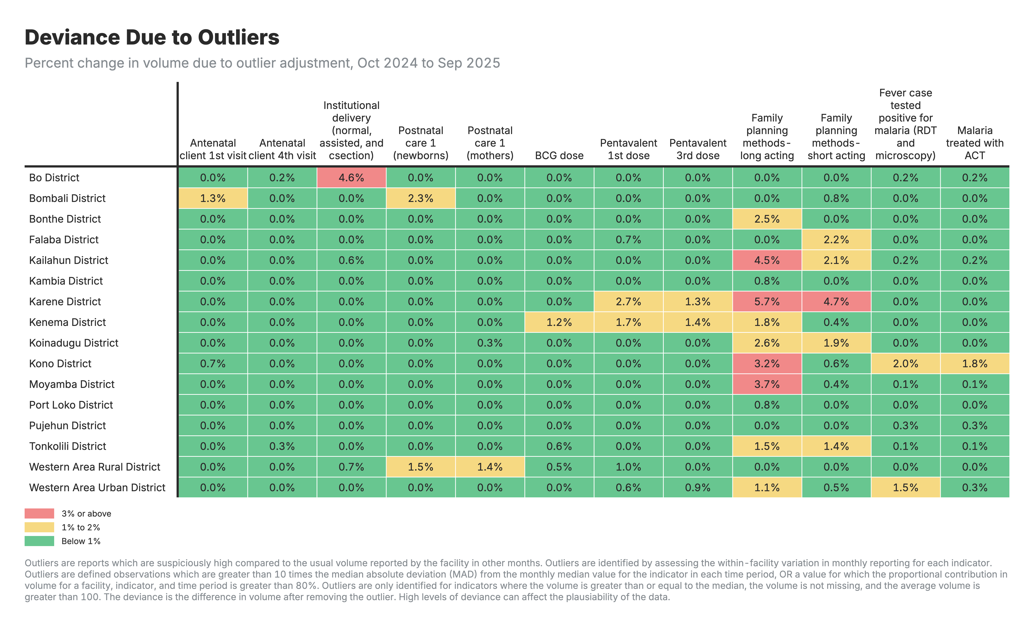
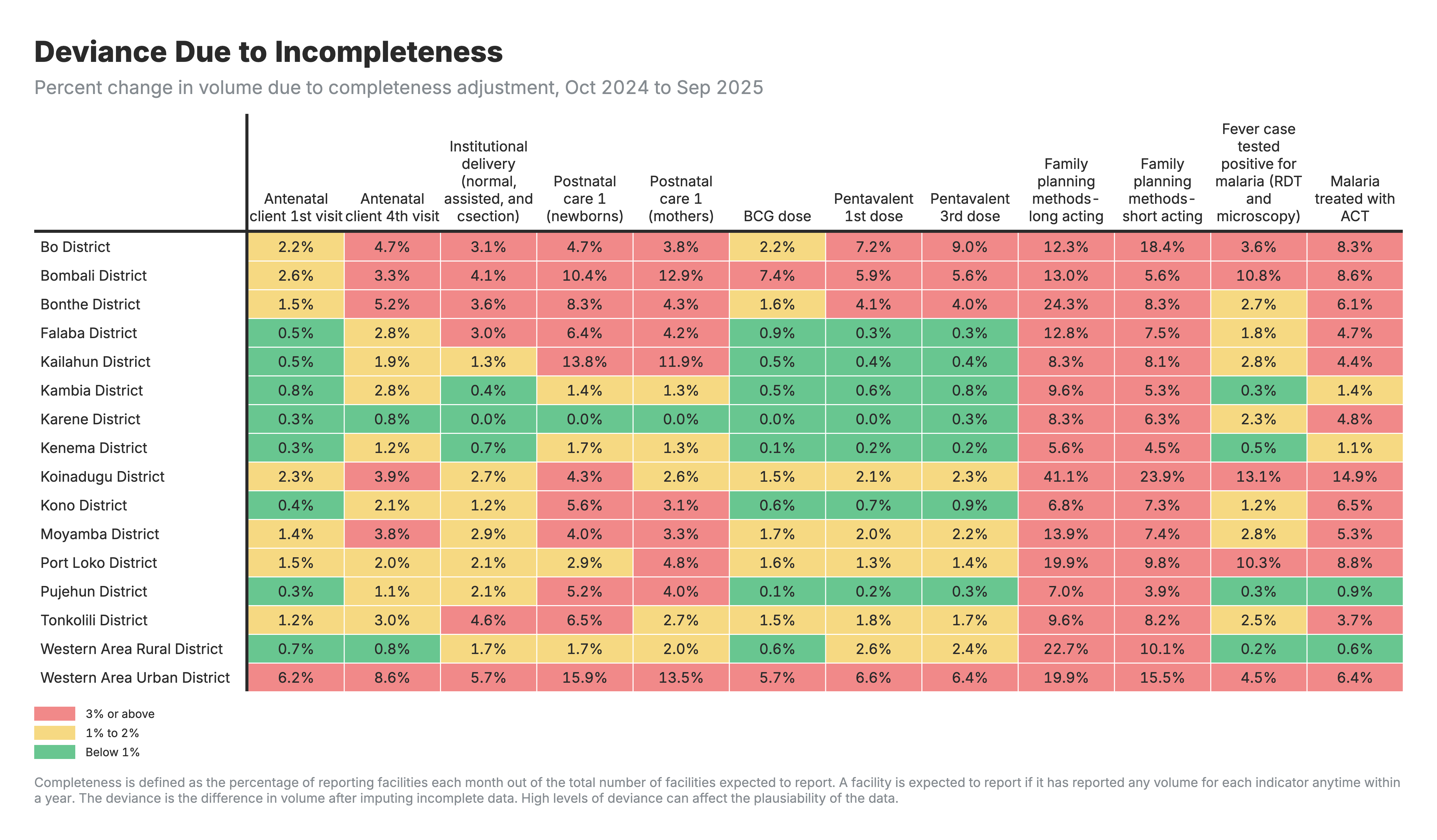
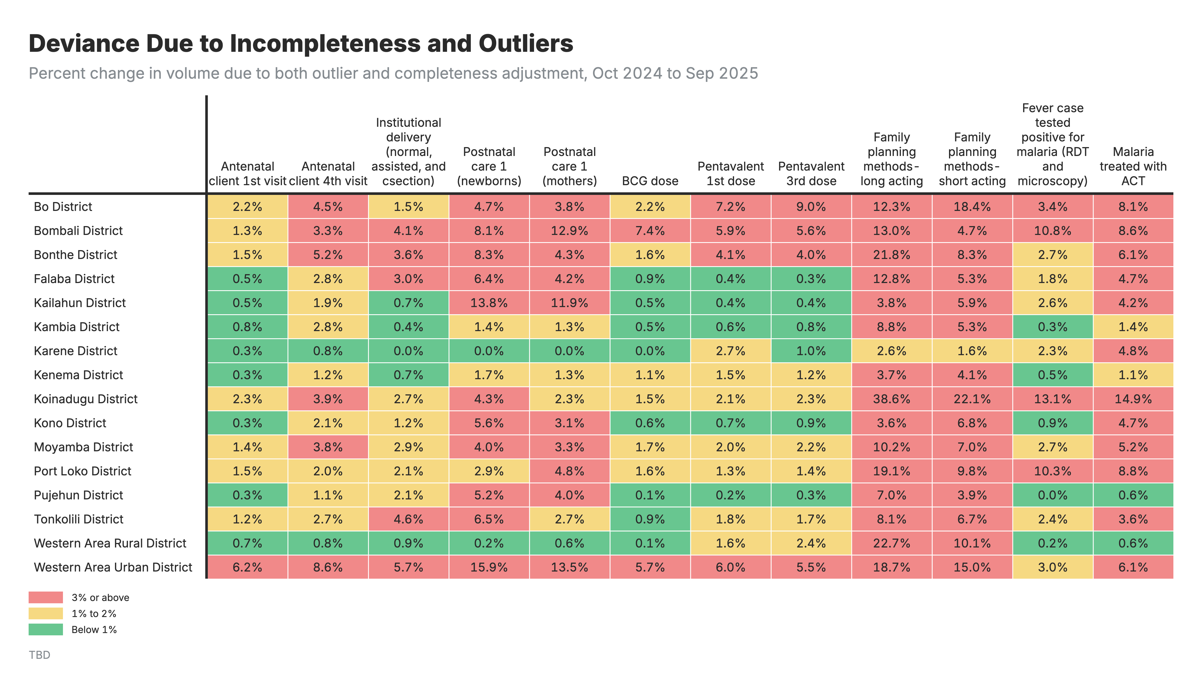
Analysis outputs and visualization

The FASTR analysis generates three main visual outputs comparing service volumes before and after adjustments:

1. Outlier adjustment impact

Heatmap showing the percent change in service volume due to outlier adjustment, by indicator and geographic area.

2. Completeness adjustment impact

Heatmap showing the percent change in service volume due to completeness (missing data) adjustment, by indicator and geographic area.

3. Combined adjustment impact

Heatmap showing the percent change in service volume when both outlier and completeness adjustments are applied.

Interpretation guide

For all heatmaps:

• Rows: Geographic areas (zones/regions)
• Columns: Health indicators
• Values: Percent change in service volume after adjustment

For the outlier adjustment heatmap (output 1):

• Negative values: Extreme high values were replaced with lower estimates
• Values near zero indicate few outliers detected

For the completeness adjustment heatmap (output 2):

• Positive values: Missing data was filled, increasing total volume
• Values near zero indicate reporting was already complete

For the combined adjustment heatmap (output 3):

• Shows net effect of both adjustments
• Negative = outlier effect dominates; Positive = completeness effect dominates

---

Detailed reference

Configuration parameters

Module m002 does not expose any user-tunable parameters in the FASTR platform — adjustments run with the same internal logic for every project. The settings documented below are hard-coded inside the module and are described here for transparency, not for configuration.

??? “Excluded indicators (hard-coded)”

Some indicators are excluded from all adjustments due to their sensitive nature. Exclusion is done via a case-insensitive regular expression match on `indicator_common_id`:

```r
EXCLUDED_PATTERN <- "death|still_birth"
```

This matches any indicator whose name contains `death` (e.g. `u5_deaths`, `maternal_deaths`, `neonatal_deaths`) or `still_birth`. For these indicators, the original raw `count` is preserved in every scenario column (`count_final_none`, `count_final_outliers`, `count_final_completeness`, `count_final_both`).

**Rationale**: Mortality and stillbirth counts should not be smoothed or imputed as they represent discrete events that may have genuine temporal variation. Adjusting these could mask important epidemiological patterns or outbreak signals.

??? “Low volume exclusions (hard-coded)”

Indicators are also automatically excluded from **adjustment** if no facility-month observation ever reaches 100 (`count >= 100`) anywhere in the dataset. This prevents meaningless statistical adjustment on indicators with consistently low counts. Excluded low-volume indicators have their raw `count` preserved across all four scenario columns, just like the excluded mortality/stillbirth indicators.

**Exclusion logic**:

```r
low_volume_check <- raw_data[, .(has_volume = any(count >= 100, na.rm = TRUE)),
                             by = indicator_common_id]
low_volume_check[, low_volume_exclude := !has_volume]
LOW_VOLUME_INDICATORS <- low_volume_check[has_volume == FALSE, indicator_common_id]
```

The full list (with a `low_volume_exclude` TRUE/FALSE flag per indicator) is saved to `M2_low_volume_exclusions.csv` for transparency.

??? “Rolling window configuration (hard-coded)“

The module uses a **6-month window** for all rolling averages. This choice balances:

**Advantages**:

- Captures medium-term trends
- Reduces impact of short-term fluctuations
- Sufficient data points for stable averages
- Works well for both stable and seasonal indicators

**Trade-offs**:

- May not capture rapid changes in service delivery
- Could over-smooth in cases of genuine programmatic shifts
- Requires at least 6 valid observations for optimal centered average

Input/output specifications

??? “Input files”

The module requires three input files from previous processing steps:

| File | Source | Description | Key Variables |
|------|--------|-------------|---------------|
| `hmis_ISO3.csv` | Raw HMIS data | Facility-level service volumes | `facility_id`, `indicator_common_id`, `period_id`, `count`, admin area columns |
| `M1_output_outliers.csv` | Module 1 | Outlier flags for each facility-month-indicator | `facility_id`, `indicator_common_id`, `period_id`, `outlier_flag` |
| `M1_output_completeness.csv` | Module 1 | Completeness flags for each facility-month-indicator | `facility_id`, `indicator_common_id`, `period_id`, `completeness_flag` |

??? “Input data structure”

**Raw HMIS Data (`hmis_ISO3.csv`)**:

```text
facility_id | admin_area_1 | admin_area_2 | admin_area_3 | period_id | indicator_common_id | count
------------|--------------|--------------|--------------|-----------|---------------------|-------
FAC001      | ISO3         | Province_A   | District_A   | 202301    | anc1                | 145
FAC001      | ISO3         | Province_A   | District_A   | 202302    | anc1                | 152
FAC001      | ISO3         | Province_A   | District_A   | 202303    | anc1                | 890  # Outlier
```

**Outlier flags (`M1_output_outliers.csv`)**:

```text
facility_id | indicator_common_id | period_id | outlier_flag
------------|---------------------|-----------|-------------
FAC001      | anc1                | 202301    | 0
FAC001      | anc1                | 202302    | 0
FAC001      | anc1                | 202303    | 1           # Flagged as outlier
```

**Completeness flags (`M1_output_completeness.csv`)**:

```text
facility_id | indicator_common_id | period_id | completeness_flag
------------|---------------------|-----------|------------------
FAC001      | anc1                | 202301    | 1             # Complete
FAC001      | anc1                | 202302    | 0             # Incomplete
FAC001      | anc1                | 202303    | 1             # Complete
```

??? “Output files”

The module generates four output files:

| File | Level | Description | Key Columns |
|------|-------|-------------|-------------|
| `M2_adjusted_data.csv` | Facility | Adjusted volumes for all scenarios at facility level | `facility_id`, admin areas (excl. admin_area_1), `period_id`, `indicator_common_id`, `count_final_*` |
| `M2_adjusted_data_admin_area.csv` | Subnational | Aggregated adjusted volumes at subnational admin areas | Admin areas (excl. admin_area_1), `period_id`, `indicator_common_id`, `count_final_*` |
| `M2_adjusted_data_national.csv` | National | Aggregated adjusted volumes at national level | `admin_area_1`, `period_id`, `indicator_common_id`, `count_final_*` |
| `M2_low_volume_exclusions.csv` | Metadata | Indicators excluded from adjustment due to low volumes | `indicator_common_id`, `low_volume_exclude` |

??? “Output data structure”

**Facility-Level Output** (`M2_adjusted_data.csv`):

```text
facility_id | admin_area_2 | admin_area_3 | period_id | indicator_common_id | count_final_none | count_final_outliers | count_final_completeness | count_final_both
------------|--------------|--------------|-----------|---------------------|------------------|----------------------|--------------------------|------------------
FAC001      | Province_A   | District_A   | 202301    | anc1                | 145              | 145                  | 145                      | 145
FAC001      | Province_A   | District_A   | 202302    | anc1                | 152              | 152                  | 148                      | 148
FAC001      | Province_A   | District_A   | 202303    | anc1                | 890              | 148                  | 890                      | 148
```

Each `count_final_*` column represents a different adjustment scenario:

- `count_final_none`: No adjustments applied (original values)
- `count_final_outliers`: Only outlier adjustment applied
- `count_final_completeness`: Only completeness adjustment applied
- `count_final_both`: Both outlier and completeness adjustments applied

Key functions documentation

??? “Required libraries”

The module depends on the following R packages:

-   `data.table` - High-performance data manipulation, aggregation, and rolling window calculations (`frollmean` for rolling averages)
-   `zoo` - Loaded for time-series utilities
-   `lubridate` - Date handling (`month()`, `year()`) used for the same-month-last-year fallback

??? “1. apply_adjustments()”

Core function that implements the adjustment logic for a single scenario.

**Purpose**:

Replaces outlier and/or incomplete values using rolling averages and historical patterns.

**Parameters**:

- `raw_data` (data.table): Original HMIS data with service counts
- `completeness_data` (data.table): Completeness flags from Module 1
- `outlier_data` (data.table): Outlier flags from Module 1
- `adjust_outliers` (logical): Whether to apply outlier adjustment
- `adjust_completeness` (logical): Whether to apply completeness adjustment

**Returns**:

data.table with adjusted values in `count_working` column and adjustment metadata

**Key operations**:

1. Merges input datasets by `facility_id`, `indicator_common_id`, and `period_id`
2. Converts `period_id` to dates for temporal ordering
3. Calculates rolling averages (centered, forward, backward) for valid values
4. Applies adjustment hierarchy based on data availability
5. Tracks adjustment method used for each replaced value

??? “2. apply_adjustments_scenarios()”

Wrapper function that runs adjustments across all four scenarios.

**Purpose**:

Applies the adjustment logic under different combinations of outlier and completeness adjustments.

**Parameters**:

- `raw_data` (data.table): Original HMIS data
- `completeness_data` (data.table): Completeness flags
- `outlier_data` (data.table): Outlier flags

**Returns**:

data.table with four `count_final_*` columns, one per scenario

**Scenarios processed**:

1. `none`: No adjustments (baseline)
2. `outliers`: Outlier adjustment only
3. `completeness`: Completeness adjustment only
4. `both`: Sequential outlier then completeness adjustment

**Processing logic**:

- Calls `apply_adjustments()` once per scenario
- Preserves the raw `count` for indicators matching the `death|still_birth` regex and for low-volume indicators (overwriting any scenario-specific `count_working`)
- Merges all scenario results into a single wide-format table with four `count_final_*` columns

Statistical methods & algorithms

??? “Outlier adjustment methodology”

Outlier adjustment is applied to any facility-month value flagged in Module 1 (`outlier_flag == 1`). The goal is to replace these outlier values using valid historical data from the same facility and indicator.

**Statistical approach**:

Rolling averages are used to estimate expected values. A rolling average (also called moving average) is the mean of a set of time periods surrounding the target period. This technique smooths short-term fluctuations and highlights longer-term trends.

**Valid values definition**:

Only values meeting ALL of the following criteria are used in calculations:

- `!is.na(count)` (non-missing)
- `outlier_flag == 0` (not flagged as outlier)

**Implementation**:

The module uses `frollmean()` from the `zoo` package for efficient rolling calculations:

```r
data_adj[, valid_count := fifelse(outlier_flag == 0L & !is.na(count), count, NA_real_)]
data_adj[, `:=`(
  roll6   = frollmean(valid_count, 6, na.rm = TRUE, align = "center"),
  fwd6    = frollmean(valid_count, 6, na.rm = TRUE, align = "left"),
  bwd6    = frollmean(valid_count, 6, na.rm = TRUE, align = "right"),
  fallback= mean(valid_count, na.rm = TRUE)
), by = .(facility_id, indicator_common_id)]
```

??? “Adjustment hierarchy for outliers”

The adjustment process follows this **hierarchical order** (stopping at the first available method):

1.  **Centered 6-Month Average (`roll6`)**

    -   Uses the three months before and three months after the outlier month
    -   Provides a balanced average based on nearby trends
    -   Applied when enough valid values exist on both sides of the month
    -   Method tag: `roll6`

2.  **Forward-Looking 6-Month Average (`fwd6`)**

    -   Used if the centered average can't be calculated (e.g. early in the time series)
    -   Takes the average of the next six valid months
    -   Method tag: `forward`

3.  **Backward-Looking 6-Month Average (`bwd6`)**

    -   Used if neither `roll6` nor `fwd6` are available
    -   Takes the average of the six most recent valid months before the outlier
    -   Method tag: `backward`

4.  **Same month from previous year**

    -   If no valid 6-month average exists, the value from the **same calendar month in the previous year** is used (e.g., Jan 2023 for Jan 2024)
    -   Only applied if that previous value is valid (not flagged as an outlier and not missing) and only when exactly one matching prior-year record is found
    -   Particularly useful for seasonal indicators (e.g., malaria, respiratory infections)
    -   Method tag: `same_month_last_year`
    -   **Implementation**:

    ```r
    data_adj[, `:=`(mm = month(date), yy = year(date))]
    data_adj <- data_adj[, {
      for (i in which(outlier_flag == 1L & is.na(adj_method))) {
        j <- which(mm == mm[i] & yy == yy[i] - 1 & outlier_flag == 0L & !is.na(count))
        if (length(j) == 1L) {
          count_working[i] <- count[j]
          adj_method[i]    <- "same_month_last_year"
          adjust_note[i]   <- format(date[j], "%b-%Y")
        }
      }
      .SD
    }, by = .(facility_id, indicator_common_id)]
    ```

5.  **Mean of All Historical Values (Fallback)**

    -   If all previous methods fail, the mean of all valid historical values for that facility-indicator is used
    -   Provides a facility-specific baseline when no temporal pattern is available
    -   Method tag: `fallback`

**Edge case**:

If even the facility-level fallback mean cannot be computed (e.g., the facility has no valid non-outlier observations at all for that indicator), the outlier value remains as `NA` in the adjusted scenario columns.

??? “Completeness adjustment methodology”

Completeness adjustment is applied to any facility-month where the working count is missing (`is.na(count_working)`). In the `completeness` scenario this is driven by the original `count` being `NA` (i.e., the facility did not report that month). In the `both` scenario, the working count may also be `NA` because the outlier step did not produce a replacement. The `completeness_flag` from Module 1 is merged in for reference but is not used as the replacement trigger.

**Statistical approach**:

The same rolling average methodology is applied, but the definition of "valid values" differs slightly:

**Valid values for completeness adjustment**:

- `!is.na(count_working)` (non-missing, possibly already adjusted for outliers)
- `outlier_flag == 0` (not flagged as outlier in original data)

**Key difference from outlier adjustment**:

- Completeness adjustment can use values that were already adjusted for outliers (when scenarios include both adjustments)
- No same-month-last-year method is used (only rolling averages and fallback)

**Implementation**:

```r
data_adj[, valid_count := fifelse(!is.na(count_working) & outlier_flag == 0L, count_working, NA_real_)]
data_adj[, `:=`(
  roll6   = frollmean(valid_count, 6, na.rm = TRUE, align = "center"),
  fwd6    = frollmean(valid_count, 6, na.rm = TRUE, align = "left"),
  bwd6    = frollmean(valid_count, 6, na.rm = TRUE, align = "right"),
  fallback= mean(valid_count, na.rm = TRUE)
), by = .(facility_id, indicator_common_id)]
```

??? “Adjustment hierarchy for completeness”

The replacement follows this **hierarchical order**:

1.  **Centered 6-Month Average (`roll6`)**

    -   Uses three valid months before and after the missing or incomplete month
    -   Preferred method when sufficient surrounding data exists
    -   Method tag: `roll6`

2.  **Forward-Looking 6-Month Average (`fwd6`)**

    -   Used if the centered average cannot be calculated (e.g., at start of time series)
    -   Method tag: `forward`

3.  **Backward-Looking 6-Month Average (`bwd6`)**

    -   Used if no centered or forward-looking values are available (e.g., at end of time series)
    -   Method tag: `backward`

4.  **Mean of All Historical Values (Fallback)**

    -   If no rolling averages can be calculated, uses the mean of all valid values for that facility-indicator
    -   Provides a facility-specific baseline
    -   Method tag: `fallback`

**Edge case**:

If the facility has no valid values at all for that indicator, the fallback mean itself is `NA` and the value remains missing in the adjusted scenario columns.

??? “Scenario processing logic”

The module processes all four adjustment scenarios simultaneously using the `apply_adjustments_scenarios()` function:

**Scenario 1: None** (`count_final_none`)

- `adjust_outliers = FALSE`, `adjust_completeness = FALSE`
- Original raw data with no modifications
- Serves as baseline for comparison

**Scenario 2: Outliers** (`count_final_outliers`)

- `adjust_outliers = TRUE`, `adjust_completeness = FALSE`
- Only outlier values are replaced
- Missing/incomplete values remain as-is
- Use case: When completeness is high but outliers are a concern

**Scenario 3: Completeness** (`count_final_completeness`)

- `adjust_outliers = FALSE`, `adjust_completeness = TRUE`
- Only missing/incomplete values are imputed
- Outliers are retained in the data
- Use case: When data quality is good but reporting is sporadic

**Scenario 4: Both** (`count_final_both`)

- `adjust_outliers = TRUE`, `adjust_completeness = TRUE`
- **Sequential processing**: Outliers adjusted first, then completeness
- Most comprehensive adjustment
- Use case: When both data quality issues are prevalent

**Processing order for "Both" scenario**:

1. Outlier adjustment creates `count_working` with outliers replaced
2. Completeness adjustment then operates on `count_working`, using the already-adjusted values
3. This ensures completeness imputation uses cleaned (non-outlier) values when available

**Important**:

After scenario-specific adjustments, excluded indicators are reset to their original raw `count`. This applies to both mortality/stillbirth indicators (matched via the `EXCLUDED_PATTERN` regex) and low-volume indicators:

```r
dat[grepl(EXCLUDED_PATTERN, indicator_common_id, ignore.case = TRUE) |
    indicator_common_id %in% LOW_VOLUME_INDICATORS, count_working := count]
```

As a result, the four `count_final_*` columns for these indicators are all equal to the raw value.

??? “Aggregation methods”

All geographic aggregations use **simple sums**:

```r
sum(count_final_both, na.rm = TRUE)
```

**Rationale**:

- Service volumes are additive (e.g., total deliveries = sum of facility deliveries)
- Missing values (`NA`) are treated as zero in aggregation
- Consistent with standard HMIS reporting practices

**Caution**:

If many facilities have `NA` values after adjustment, subnational/national totals may be underestimated. The `count_final_none` scenario provides a reference point for assessing impact.

??? “Handling missing data in calculations”

The module applies `na.rm = TRUE` in all rolling calculations:

```r
frollmean(valid_count, 6, na.rm = TRUE, align = "center")
```

**Implication**:

Rolling averages are calculated from available valid values only. If fewer than 6 values exist, the average is computed from whatever is available. If no valid values exist, the result is `NA`.

Code examples

??? “Example 1: Outlier adjustment”

**Scenario**:

A facility reports an unusually high first antenatal care visit (ANC1) count in March 2023.

**Data**:

```text
period_id | count | outlier_flag | Surrounding valid values
----------|-------|--------------|-------------------------
202301    | 145   | 0            | valid
202302    | 152   | 0            | valid
202303    | 890   | 1            | OUTLIER
202304    | 148   | 0            | valid
202305    | 155   | 0            | valid
202306    | 147   | 0            | valid
```

**Adjustment calculation** (centered 6-month average):

- Valid values: [145, 152, 148, 155, 147] (excludes outlier 890)
- Average: (145 + 152 + 148 + 155 + 147) / 5 = 149.4
- **Adjusted value**: 149.4

**Method used**:

`roll6`

??? “Example 2: Completeness adjustment”

**Scenario**:

A facility fails to report malaria tests in February 2023.

**Data**:

```text
period_id | count | completeness_flag | Surrounding valid values
----------|-------|-------------------|-------------------------
202301    | 45    | 1                 | valid
202302    | NA    | 0                 | INCOMPLETE
202303    | 48    | 1                 | valid
202304    | 52    | 1                 | valid
202305    | 50    | 1                 | valid
```

**Adjustment calculation** (centered 6-month average):

- Valid values: [45, 48, 52, 50, ...]
- Average: 48.75 (using available surrounding months)
- **Imputed value**: 48.75

**Method used**:

`roll6`

??? “Example 3: Seasonal indicator with same-month-last-year”

**Scenario**:

Malaria cases show strong seasonality, and a June 2023 outlier needs adjustment.

**Data**:

```text
period_id | count | outlier_flag | Notes
----------|-------|--------------|-------
202206    | 234   | 0            | June 2022 (valid)
202306    | 1850  | 1            | June 2023 (OUTLIER)
```

**Adjustment logic**:

1. Centered, forward, and backward rolling averages unavailable (insufficient data)
2. Same-month-last-year method activated
3. June 2022 value = 234 (valid)
4. **Adjusted value**: 234

**Method used**:

`same_month_last_year`

??? “Example 4: Scenario comparison”

**Facility**:

FAC001

**Indicator**:

Institutional deliveries

**Period**:

Q1 2023

**Original data**:

```text
Month    | Count | Outlier? | Complete?
---------|-------|----------|----------
Jan 2023 | 78    | No       | Yes
Feb 2023 | 450   | Yes      | Yes       # Outlier
Mar 2023 | NA    | -        | No        # Incomplete
```

**Scenario results**:

| Month    | None | Outliers | Completeness | Both |
|----------|------|----------|--------------|------|
| Jan 2023 | 78   | 78       | 78           | 78   |
| Feb 2023 | 450  | 82*      | 450          | 82*  |
| Mar 2023 | NA   | NA       | 80**         | 80** |

*Adjusted using rolling average

**Imputed using rolling average

**Interpretation**:

- **None**: Raw data with obvious issues
- **Outliers**: February corrected, but March remains missing
- **Completeness**: March filled in, but February outlier retained
- **Both**: Most complete and clean dataset

??? “Example 5: Geographic aggregation”

**Subnational aggregation code**:

```r
adjusted_data_admin_area_final <- adjusted_data_export[
  ,
  .(
    count_final_none         = sum(count_final_none,         na.rm = TRUE),
    count_final_outliers     = sum(count_final_outliers,     na.rm = TRUE),
    count_final_completeness = sum(count_final_completeness, na.rm = TRUE),
    count_final_both         = sum(count_final_both,         na.rm = TRUE)
  ),
  by = c(geo_admin_area_sub, "indicator_common_id", "period_id")
]
```

**National aggregation code**:

```r
adjusted_data_national_final <- adjusted_data_export[
  ,
  .(
    count_final_none         = sum(count_final_none,         na.rm = TRUE),
    count_final_outliers     = sum(count_final_outliers,     na.rm = TRUE),
    count_final_completeness = sum(count_final_completeness, na.rm = TRUE),
    count_final_both         = sum(count_final_both,         na.rm = TRUE)
  ),
  by = .(admin_area_1, indicator_common_id, period_id)
]
```

Troubleshooting

??? “Common issues”

**Issue 1: All values remain unadjusted**

**Possible causes**:

- Indicator name matches the `death|still_birth` exclusion pattern
- Indicator flagged as low-volume (no observation ever reached `count >= 100`)
- No outlier flags (`outlier_flag == 1`) and no missing values in the input data

**Solution**:

Check `M2_low_volume_exclusions.csv` and verify Module 1 outputs contain flags

**Issue 2: Adjusted values seem unreasonable**

**Possible causes**:

- Insufficient valid historical data for rolling averages
- Genuine program changes being smoothed out
- Seasonal patterns not captured by 6-month window

**Solution**:

- Review facility-specific time series plots
- Consider using "outliers only" scenario if completeness is good
- Validate against program implementation records

**Issue 3: Many NA values after adjustment**

**Possible causes**:

- Facility has very sparse data
- No valid values available for any adjustment method
- Early months in time series lack historical data

**Solution**:

- Expected for facilities with limited reporting history
- Consider facility-level data quality filtering
- National/subnational aggregates will sum available values

**Issue 4: Subnational/national totals don't match expectations**

**Possible causes**:

- NA values treated as zero in aggregation
- Different scenarios produce different totals
- Low reporting completeness overall

**Solution**:

- Compare `count_final_none` vs `count_final_both` to assess adjustment impact
- Review Module 1 completeness statistics
- Consider data quality threshold for inclusion

??? “Quality assurance checks”

The module includes several quality checks:

1. **Low volume exclusions**: Automatically identifies and excludes indicators that never reach `count >= 100`
2. **Adjustment tracking**: Counts and reports the number of values adjusted by each method (`roll6`, `forward`, `backward`, `same_month_last_year`, `fallback`)
3. **Excluded indicators**: Ensures mortality and stillbirth indicators (matched via `death|still_birth` regex) are never adjusted
4. **Console logging**: Provides detailed progress and summary statistics

**Example console output**:

```text
Running adjustments...
 -> Adjusting outliers...
     Roll6 adjusted: 1,245
     Forward-filled: 89
     Backward-filled: 67
     Same-month LY: 34
     Fallback mean: 12
 -> Adjusting for completeness...
     Roll6 filled: 2,103
     Forward-filled: 234
     Backward-filled: 178
     Fallback mean: 45
```

Usage notes

??? “Choosing the right scenario”

| Situation | Recommended Scenario | Rationale |
|-----------|---------------------|-----------|
| High data quality, minimal issues | `none` | No adjustment needed |
| Sporadic outliers, good completeness | `outliers` | Address quality without imputation |
| Good quality, poor reporting frequency | `completeness` | Fill gaps while preserving actual values |
| Poor quality and completeness | `both` | Comprehensive cleaning |
| Uncertainty about data quality | Compare all scenarios | Sensitivity analysis |

??? “Validation steps”

After running this module, consider:

1. **Compare scenarios**: Examine differences between `count_final_none` and `count_final_both`
2. **Review exclusions**: Check `M2_low_volume_exclusions.csv` for unexpected indicators
3. **Aggregate analysis**: Ensure subnational and national totals are reasonable
4. **Temporal plots**: Visualize trends before/after adjustment to identify over-smoothing
5. **Facility-level spot checks**: Review adjustments for a sample of facilities

??? “Limitations”

1. **Rolling windows assume stability**: Adjustments work best when service delivery is relatively stable. Genuine program changes (e.g., new campaigns) may be incorrectly smoothed.

2. **No adjustment uncertainty**: The module provides point estimates without confidence intervals. Adjusted values should be treated as estimates.

3. **Facility-specific adjustments**: No cross-facility borrowing of information. Facilities with very sparse data may have unstable adjustments.

4. **Seasonal patterns**: While same-month-last-year helps, strong within-year seasonality may not be fully captured by 6-month windows.

5. **NA treatment in aggregation**: Missing values are treated as zero when summing to higher geographic levels, which may underestimate totals if missingness is high.

---

Contact: fastr@worldbank.org

---

Rationale for data quality adjustment

Routine HMIS data contain two common limitations that can distort analytical results:

• Outliers: Extreme values create artificial spikes in service volumes
• Incomplete reporting: Missing data creates artificial declines that do not reflect actual service delivery

FASTR addresses these limitations by replacing problematic values with estimates derived from each facility’s historical reporting patterns.

Adjustment scenarios: To support transparency and sensitivity analysis, FASTR produces four parallel datasets:

• Unadjusted: Original reported values
• Outliers adjusted: Extreme values replaced
• Completeness adjusted: Missing values imputed
• Both adjusted: All corrections applied

Outlier adjustment methodology

Outlier values are replaced using facility-specific historical data. The adjustment follows a hierarchical approach:

Priority	Method	Application
1	Centered 6-month average	3 months before + 3 months after the outlier
2	Forward 6-month average	When insufficient preceding data (e.g., start of series)
3	Backward 6-month average	When insufficient following data (e.g., end of series)
4	Same month, previous year	When rolling averages unavailable; useful for seasonal indicators
5	Facility historical mean	Mean of all valid values for this indicator at this facility

Completeness adjustment methodology

For months identified as incomplete or missing, values are imputed using the same 6-month rolling average approach applied to outlier adjustment.

Priority	Method	Application
1	Centered 6-month average	When sufficient data exists before and after the gap
2	Forward 6-month average	For gaps at the start of the time series
3	Backward 6-month average	For gaps at the end of the time series
4	Facility historical mean	Mean of all valid values for this indicator at this facility

This approach prevents temporary reporting gaps from creating artificial declines in service volumes.

Data quality adjustment

Why adjust? Outliers and reporting gaps identified in the DQA will distort service utilization and coverage estimates if left uncorrected. The goal is to replace problematic values with reasonable estimates based on each facility’s own historical patterns.

How? Outliers and missing values are replaced using 6-month rolling averages from the facility’s historical data.

Four parallel datasets: FASTR produces unadjusted, outliers-only adjusted, completeness-only adjusted, and both-adjusted versions. This enables sensitivity analysis - comparing results across scenarios to assess how much conclusions depend on adjustment choices.

Excluded from adjustment: Mortality indicators (discrete events that shouldn’t be smoothed) and low-volume indicators (<100 events/month, where adjustment adds noise).

Why adjust for outliers?

Outlier adjustment output

What you see: Heatmap showing how much service volume changed after replacing outliers with rolling averages.

Formula: % change = (adjusted - original) / original × 100

Interpretation: Values are typically negative (outliers removed reduce volume). Large adjustments warrant investigation into their source.

Indicators excluded from adjustment

Certain indicators are excluded from the adjustment process:

• Mortality indicators (maternal deaths, neonatal deaths, under-5 deaths): These represent discrete events where smoothing or imputation is not appropriate
• Low-volume indicators: Indicators that never exceed 100 reported events in any month are excluded from adjustment

Data correction: how FASTR fixes problems

Rather than throwing away problematic data, FASTR replaces it with reasonable estimates — like replacing a faulty meter reading with the average of surrounding months.

Extreme values → Replaced by the average of the 6 months around them Missing months → Filled in with the facility’s historical trend

FASTR produces 4 versions of the data for comparison:

Version	What it contains
Raw data	No modifications
Outliers corrected	Extreme spikes smoothed
Completeness adjusted	Missing months filled
Both adjustments	Spikes smoothed + missing months filled

You can compare results across all 4 versions. If your conclusions change, that’s a signal that data quality deserves attention.

Completeness adjustment output

What you see: Heatmap showing how much service volume changed after imputing missing data with rolling averages.

Formula: % change = (adjusted - original) / original × 100

Interpretation: Values are typically positive (imputation adds volume). Large adjustments indicate areas needing completeness improvement.