Coverage estimates

Background and purpose

Objective of the module

The Coverage Estimates module quantifies health service coverage by integrating adjusted administrative service volumes from the Health Management Information System (HMIS), population projections from the United Nations World Population Prospects (UN WPP), and household survey data. While the module currently draws on Demographic and Health Surveys (DHS) and Multiple Indicator Cluster Surveys (MICS), it is designed to accommodate other nationally representative survey sources as they become available. The module estimates the share of the target population that received a given health service, providing a standardized measure of service reach for use in monitoring, comparison, and downstream analysis. The module is structured in two components.

Part 1 constructs target population denominators using multiple methodological approaches and evaluates their performance by comparing resulting coverage estimates with available survey reference values for each health indicator.

Part 2 allows users to review and adjust denominator selections based on programmatic considerations and to extend survey-based coverage estimates over time using trends derived from administrative data, where survey data are not available.

Together, these components convert administrative service volumes into standardized coverage estimates that can be examined over time and across geographic levels, and used in analytical and monitoring contexts.

Analytical rationale

Health service coverage is a core metric for assessing health system performance and equity. While Module 2 produces adjusted service volumes, these figures on their own do not indicate the extent to which services reach the populations they are intended to serve. Coverage estimates place service delivery in context by relating service volumes to population need.

This module addresses key challenges in estimating coverage, including:

• Multiple data sources: Integrates HMIS data with survey data

• Denominator uncertainty: Different methods for estimating target populations may yield different results; the module systematically evaluates options

• Temporal gaps: Surveys occur every 3-5 years; the module projects estimates for intervening years using administrative trends

• Subnational analysis: Enables coverage monitoring at national, provincial, and district levels

Key points

Component	Details
Inputs	M2_adjusted_data (national & subnational) from Module 2 Survey data (MICS/DHS) from GitHub repository Population data (UN WPP) from GitHub repository
Outputs	M5 (Part 1) — M5_denominators (national, admin2, admin3): calculated target populations · M5_combined_results (national, admin2, admin3): coverage estimates with all denominators · M5_selected_denominator_per_indicator: best denominator per indicator and level M6 (Part 2) — M6_coverage_estimation (national, admin2, admin3): final coverage with HMIS, survey, and projected estimates
Module IDs	Part 1 = m005 (requires m002) · Part 2 = m006 (requires m005)
Purpose	Estimate health service coverage by comparing service volumes to target populations, validated against survey benchmarks

!!! warning “Reminder: HMIS input must be counts, not coverage %“

Coverage estimation works by dividing the number of services delivered (the **count** flowing through Modules 1, 2, and 3) by a target-population denominator that the platform builds itself. If your original HMIS extract contained pre-calculated coverage rates instead of service counts, there is nothing for this module to compute — the count is the numerator, and the platform supplies the denominator. See [Data extraction](02_data_extraction) for what to pull from your HMIS.

Part 1 and part 2 explained

Coverage estimation is split across two modules that always run in sequence: m005 (Part 1) produces every denominator option, and m006 (Part 2) picks one denominator chain and turns it into final coverage estimates.

Part 1 — m005 denominator calculation and chain pre-selection

• Requires: m002 (adjusted HMIS data)

• Calculates target populations (denominators) using multiple approaches: HMIS-based (from ANC1, delivery, BCG, Penta1, live births) and population-based (UN WPP)

• Compares each HMIS-based chain to UN WPP and pre-selects the chain whose median ratio is closest to 1.0 (the best chain) — this is one chain applied to all indicators, not a per-indicator pick

• Outputs all denominator values, plus a M5_combined_results_*.csv per geographic level with coverage estimated using every available denominator, the best chain’s coverage, and the raw survey values

• Outputs: M5_denominators_national.csv, M5_denominators_admin2.csv, M5_denominators_admin3.csv, M5_combined_results_national.csv, M5_combined_results_admin2.csv, M5_combined_results_admin3.csv, M5_selected_denominator_per_indicator.csv

Part 2 — m006 denominator chain selection and survey projection

• Requires: m005 (M5_combined_results_*.csv for national / admin2 / admin3)

• Single user parameter DENOMINATOR_CHAIN (auto, anc1, delivery, bcg, penta1) — auto keeps the chain pre-selected by m005; any other value forces a single chain across all indicators and all geographic levels

• Computes year-over-year coverage deltas from the selected chain and projects the most recent survey value forward using those deltas (additive method)

• Outputs: M6_coverage_estimation_national.csv, M6_coverage_estimation_admin2.csv, M6_coverage_estimation_admin3.csv — each row carries HMIS coverage, original survey value, and projected survey value side by side

---

Analytical workflow

Overview of analytical steps

Part 1: Denominator calculation and selection

Step 1: Load and prepare data sources The module begins by loading three data sources and ensuring they are compatible. HMIS data is aggregated from monthly to annual totals. Survey data is harmonized (DHS prioritized over MICS) and forward-filled to create continuous time series. Population data is filtered to the target country.

Step 2: Calculate multiple denominator options For each health indicator, the module calculates several possible target populations:

• Service-based denominators: Using HMIS volumes divided by survey coverage (e.g., if 10,000 women received ANC1 and survey says coverage is 80%, estimated pregnancies = 10,000/0.80 = 12,500)

• Population-based denominators: Using UN population projections and birth rates

• Each denominator is adjusted for demographic factors (pregnancy loss, stillbirths, mortality rates) to match the indicator’s target age group

Step 3: Calculate coverage for each denominator The module computes coverage by dividing the service volume by each denominator option. This produces multiple coverage estimates per indicator, each based on a different population assumption.

Step 4: Pre-select a single denominator chain At national level, the module compares each HMIS-based chain (ANC1, delivery, Penta1) to UN WPP population estimates for the same target populations (pregnancies, live births, infants eligible for DPT). For each chain it computes the median ratio of chain values to UN WPP values, then picks the chain whose median ratio is closest to 1.0. The BCG chain is national-only and is excluded from the auto comparison (it can still be forced as a manual override). UN WPP serves as an independent demographic anchor, not as the “best” coverage value.

Step 5: Apply the chain across geographies The same chain selected at national level is reused for admin area 2 and admin area 3, ensuring that one consistent source feeds every geography. If the chain is national-only (BCG), subnational rows are dropped from that output.

Step 6: Generate outputs The module saves: per-indicator denominator values (M5_denominators_*.csv); combined results (M5_combined_results_*.csv) holding coverage for every denominator option, the best chain entries used by m006, and the raw survey values; and a summary table (M5_selected_denominator_per_indicator.csv) listing which denominator the chain assigns to each indicator at each level.

Step 7: Repeat for subnational levels If subnational data is available, the process repeats for administrative level 2 (e.g., provinces) and level 3 (e.g., districts), with fallback mechanisms to handle missing local survey data.

Part 2: Denominator selection and survey projection

Step 1: User configuration The user sets one parameter, DENOMINATOR_CHAIN. The default auto keeps Part 1’s pre-selected chain (the best rows in M5_combined_results_*.csv). Any other value (anc1, delivery, bcg, penta1) forces that single chain to be used for every indicator and every geographic level.

Step 2: Filter to the selected chain The module reads M5_combined_results_*.csv and keeps only the rows belonging to the selected chain, dropping the raw survey rows. This produces one coverage value per indicator × year × geography.

Step 3: Calculate coverage trends Year-over-year changes (deltas) in HMIS-based coverage are calculated. This shows whether coverage is increasing, decreasing, or stable over time.

Step 4: Identify survey baseline For each geographic area and indicator, the most recent survey observation is identified as the baseline anchor point for projections.

Step 5: Project survey estimates forward The module extends survey coverage estimates into years without surveys by applying HMIS trends. The projection uses: Last survey value + (Current year HMIS coverage - Survey year HMIS coverage). This preserves the survey calibration while incorporating observed trends.

Step 6: Combine all estimates The final output merges three types of estimates:

• HMIS-based coverage: Direct calculation from service volumes and selected denominators

• Original survey values: Actual household survey observations

• Projected survey coverage: Survey estimates extended using HMIS trends

Step 7: Save final outputs Results are saved with standardized column structures for each administrative level, ready for visualization and reporting.

Workflow diagram

Key decision points

1. Selection of denominators

In Part 1 (m005), the module compares each HMIS-based denominator chain to UN WPP population estimates and pre-selects the chain whose median ratio to UN WPP is closest to 1.0. The same chain is then applied to every indicator and every geographic level for consistency. In Part 2 (m006), the user can either keep this auto-selected chain or force a specific chain (anc1, delivery, bcg, or penta1). The choice determines whether coverage estimates are primarily anchored to one set of HMIS service-based denominators (e.g., everything derived from ANC1 visits) or another (e.g., everything derived from Penta1 doses).

2. Treatment of gaps between surveys

Household surveys are conducted at irregular intervals, typically every three to five years. In Part 1, survey values are forward-filled between survey years, implicitly assuming constant coverage until the next survey observation. In Part 2, coverage is projected forward using trends derived from HMIS data, allowing changes in service delivery to be reflected in periods without survey data.

3. Use of national versus subnational survey data

Coverage estimation at subnational levels requires both subnational HMIS service volumes (from Module 2) and subnational survey reference values (DHS/MICS). The module handles missing inputs at two distinct points:

• No subnational HMIS data for the country — when M2_adjusted_data_admin_area.csv contains no usable subnational rows, or when no subnational survey data exists at all in the unified DHS/MICS dataset for the country, Part 1 falls back to NATIONAL_ONLY and Part 2 detects empty admin2/admin3 M5_combined_results_*.csv files and skips the corresponding block entirely. In that case M6_coverage_estimation_admin2.csv and/or M6_coverage_estimation_admin3.csv are still written, but as empty files with the correct column headers only.

• Subnational HMIS present but a given indicator has no subnational survey value — the module does not carry the national survey value down to subnational areas as a substitute. The corresponding *carry column is left as NA for that geography-indicator-year, so no HMIS-implied denominator can be computed for that indicator at that level, and the indicator simply does not appear in subnational coverage outputs.

• Chain pre-selection has no admin2/admin3 result — when m005 cannot identify a best chain at national level (no overlapping HMIS and UN WPP data), the denominator-per-indicator entries fall back to NOT_AVAILABLE. When the selected chain is national-only (BCG), denominator_admin2 and denominator_admin3 in M5_selected_denominator_per_indicator.csv are explicitly set to NOT_AVAILABLE and no subnational rows are produced for that chain.

Indicator-level fallbacks within the survey dataset itself are narrower and remain in place at every geographic level: when SBA is absent, the module reuses the delivery survey value; when pnc1_mother is absent, it reuses the pnc1 survey value.

4. Adjustment of denominators for target populations

Each health indicator corresponds to a specific target population (for example, pregnant women for antenatal care or infants for childhood vaccination). The module applies sequential demographic adjustments—such as pregnancy loss, stillbirths, and mortality—to align denominators with the relevant target population for each indicator.

Data processing and outputs

Input integration

The module integrates three primary data sources: annualized HMIS service volumes aggregated by geographic unit; household survey coverage estimates harmonized across survey rounds and forward-filled to create continuous time series; and population projections filtered to extract age- and sex-specific populations relevant to each health indicator.

Denominator construction

Using the relationship between reported HMIS service volumes and survey-based coverage estimates, the module derives HMIS-implied denominators representing the population size consistent with observed service delivery and survey coverage levels. These denominators are further adjusted to reflect indicator-specific target populations through sequential demographic corrections, including pregnancy loss, stillbirths, and mortality.

Coverage calculation

Multiple coverage estimates are calculated by dividing service volumes by alternative denominator options, including population-based and HMIS-implied approaches. Squared error against carried-forward survey values is computed for diagnostic transparency, while the actual chain selection in m005 is driven by proximity to UN WPP at the national level.

Temporal projection

For years beyond the most recent survey observation, coverage estimates are projected forward by combining the last observed survey value with trends derived from HMIS data.

---

Analysis outputs and visualization

The FASTR analysis generates coverage estimate visualizations at multiple geographic levels:

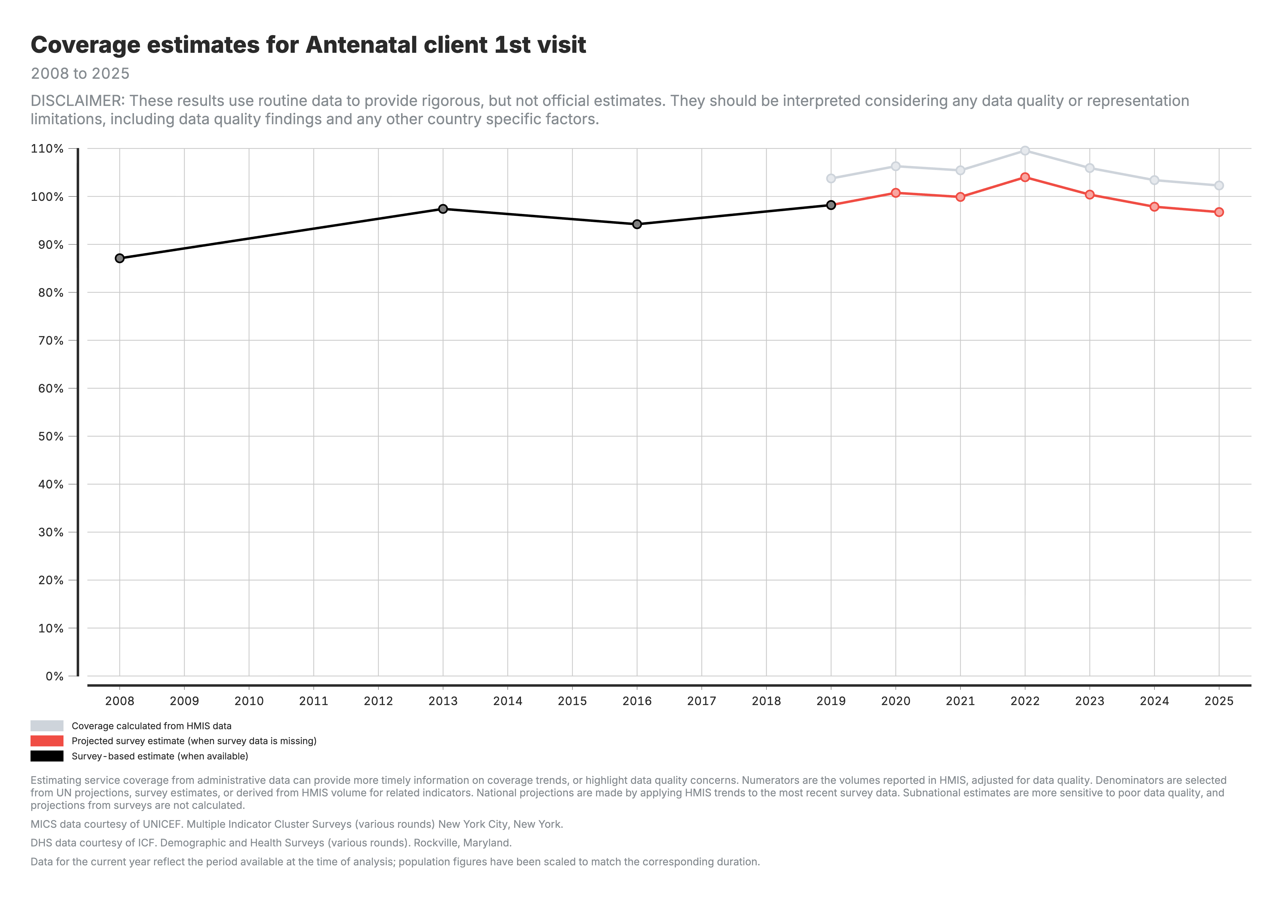
1. Coverage calculated from HMIS data (national)

National-level coverage trends comparing HMIS-derived estimates against survey benchmarks.

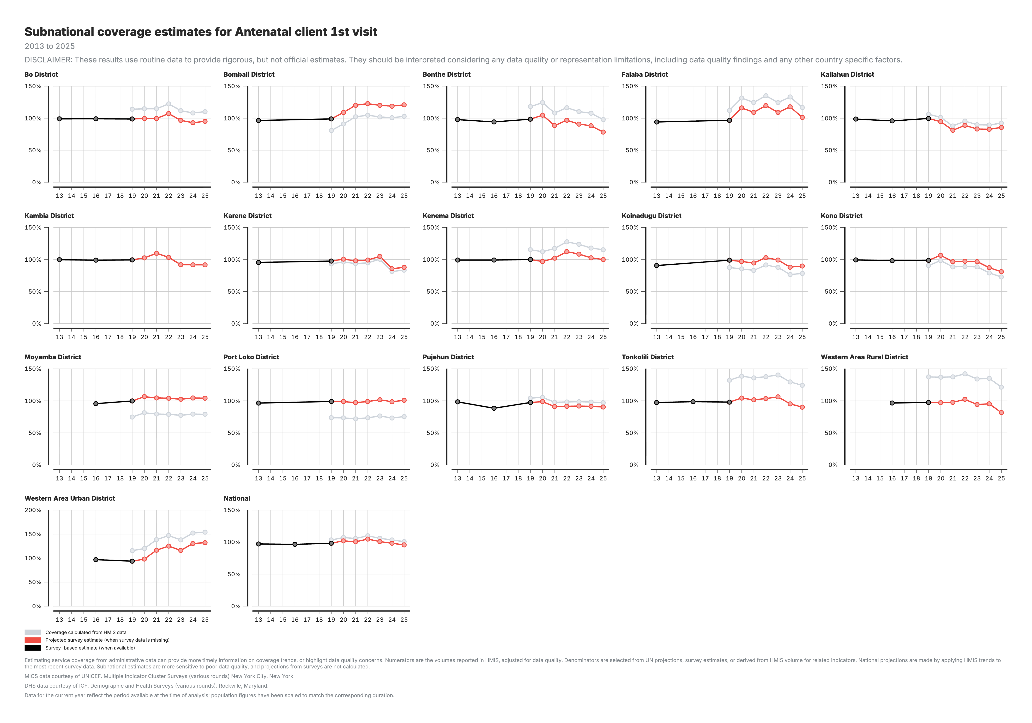
2. Coverage calculated from HMIS data (admin area 2)

Coverage patterns at an intermediate subnational level (admin_area_2), highlighting geographic variation in service delivery across regions.

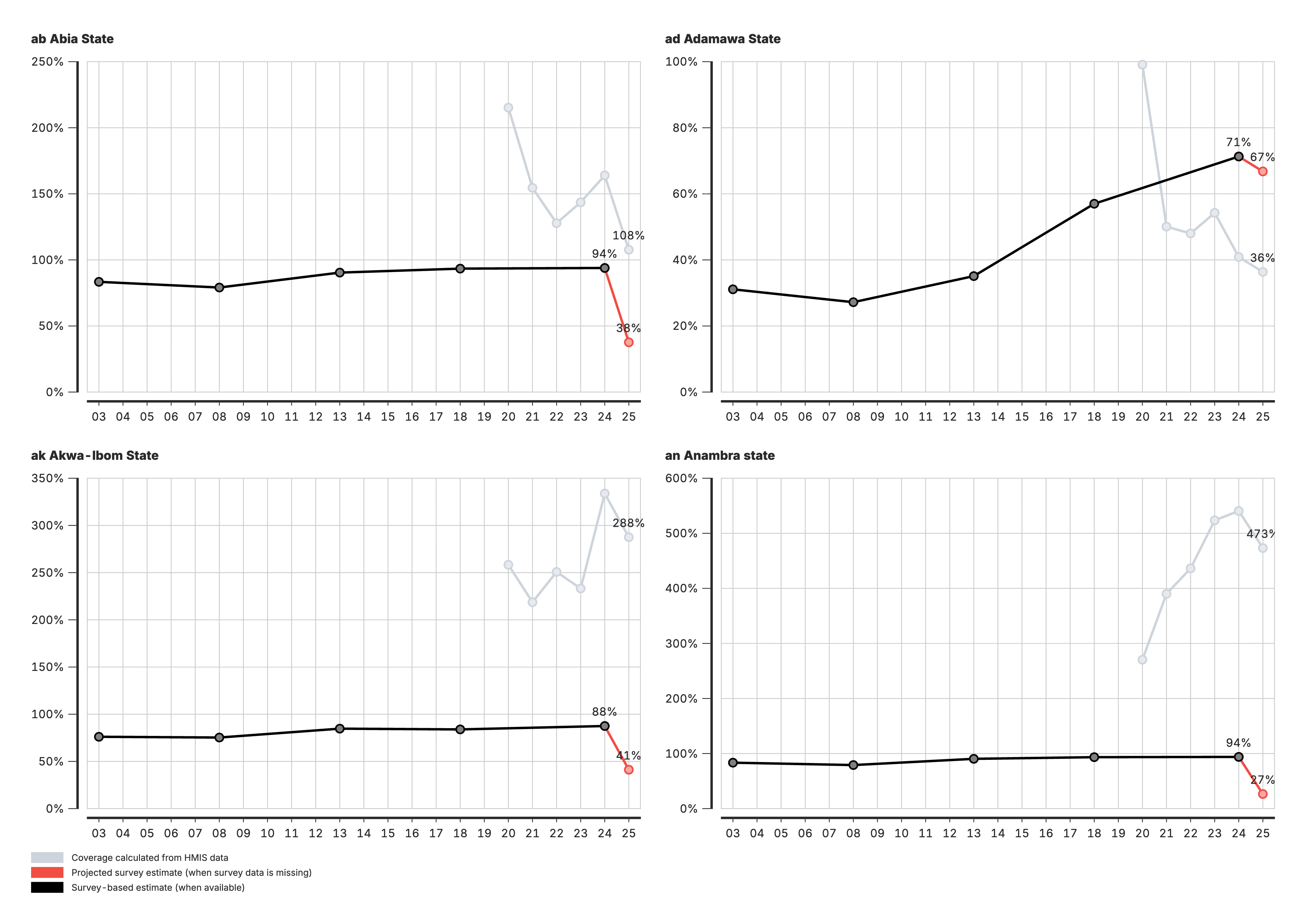
3. Coverage calculated from HMIS data (admin area 3)

Coverage estimates at a finer subnational level (admin_area_3), supporting more localized monitoring and identification of subnational disparities.

Interpretation guide

For all coverage charts (outputs 1–3):

• Black line/points: Survey-based coverage (DHS/MICS) — the reference standard
• Grey line/points: HMIS-based coverage calculated from facility data
• Red line/points: Projected coverage extending survey estimates using HMIS trends
• Y-axis: Coverage percentage (0–100%)
• X-axis: Time period (years)

Geographic levels:

• Output 1: National-level trends
• Output 2: Admin area 2 (regional/provincial) breakdown
• Output 3: Admin area 3 (district) breakdown for local targeting

---

Detailed reference

Part 1: Denominator calculation (technical details)

Configuration parameters

The module begins with several configurable parameters that control the analysis:

COUNTRY_ISO3 <- "ISO3"                         # ISO3 country code (e.g., "RWA", "UGA", "ZMB")
SELECTED_COUNT_VARIABLE <- "count_final_both"  # Which adjusted count to use
ANALYSIS_LEVEL <- "NATIONAL_PLUS_AA2"          # Geographic scope

Analysis level options:

• NATIONAL_ONLY: National-level analysis only
• NATIONAL_PLUS_AA2: National + administrative area 2 (e.g., provinces)
• NATIONAL_PLUS_AA2_AA3: National + admin area 2 + admin area 3 (e.g., districts)

Demographic adjustment rates:

PREGNANCY_LOSS_RATE <- 0.03      # 3% pregnancy loss
TWIN_RATE <- 0.015               # 1.5% twin births
STILLBIRTH_RATE <- 0.02          # 2% stillbirths
P1_NMR <- 0.039                  # Neonatal mortality rate
P2_PNMR <- 0.028                 # Post-neonatal mortality rate
INFANT_MORTALITY_RATE <- 0.067   # Infant mortality rate
UNDER5_MORTALITY_RATE <- 0.103   # Under-5 mortality rate

Count variable options:

• count_final_none: No adjustments (raw reported data)
• count_final_outliers: Outlier adjustment only (default)
• count_final_completeness: Completeness adjustment only
• count_final_both: Both adjustments combined

Input data sources

Part 1 integrates three primary data sources:

1. HMIS Adjusted Data (from Module 2)

• National: M2_adjusted_data_national.csv
• Subnational: M2_adjusted_data_admin_area.csv
• Contains service volumes by indicator, area, and time period

2. Survey Data (DHS/MICS)

• Source: GitHub repository (unified survey dataset)
• Provides coverage benchmarks for comparison
• DHS data prioritized over MICS when both available

3. Population Data (UN WPP)

• Source: GitHub repository
• Provides population-based denominators
• Includes total population, births, under-1, and under-5 populations

Additional data context:

Population projections (UN WPP) Sourced from the United Nations World Population Prospects, these estimates provide age-specific and total population figures used to calculate denominators for coverage estimates. These projections account for demographic trends, including fertility, mortality, and migration.

Survey data - MICS MICS, conducted by UNICEF, provide household survey-based estimates for key health indicators, including coverage of maternal and child health services.

Survey data - DHS DHS, conducted by USAID, provide survey data on health service utilization, including immunization rates and maternal care coverage.

Core functions documentation

??? “process_hmis_adjusted_volume()”

**Purpose**: Prepares HMIS data for denominator calculation

**Input**:

- Adjusted volume data from Module 2
- Selected count variable (e.g., `count_final_both`)

**Processing**:

- Aggregates monthly data to annual totals
- Counts number of reporting months per year
- Pivots data to wide format (one column per indicator)

**Output**:

- `annual_hmis`: Annual service counts by area and year
- `hmis_countries`: List of countries in dataset
- `hmis_iso3`: ISO3 code(s) present

**Example structure**:

```
admin_area_1  admin_area_2  year  countanc1  countdelivery  ...  nummonth
Country_Name  Province_A    2020  12500      10200          ...  12
Country_Name  Province_A    2021  13000      10500          ...  11
```

??? “process_survey_data()”

**Purpose**: Harmonizes and extends survey data for use as coverage benchmarks

**Input**:

- Survey data (DHS/MICS)
- HMIS country names and ISO3 codes
- Optional national reference (for subnational fallback)

**Key processing steps**:

1. **Harmonization**
   - Recodes indicator names (e.g., `polio1` → `opv1`, `vitamina` → `vitaminA`)
   - Normalizes source labels (`dhs`, `mics`)
   - Filters by country and date range

2. **Source prioritization**
   - When both DHS and MICS exist for same year/area/indicator
   - DHS is selected preferentially
   - Preserves source details for transparency

3. **Fallback logic**
   - If `sba` missing, uses `delivery` values
   - If `pnc1_mother` missing, uses `pnc1` values
   - At subnational levels, missing survey values for any indicator are left as `NA` — no national value is substituted (gaps are reported in the run log per indicator)

4. **Forward-Filling**
   - Creates complete time series for each area
   - Carries forward last observed value (`na.locf`)
   - Creates "carry" columns (e.g., `anc1carry`, `bcgcarry`)

**Output**:

- `carried`: Extended survey data with forward-filled values
- `raw`: Raw survey observations (wide format)
- `raw_long`: Raw survey observations (long format) with source details

??? “process_national_population_data()”

**Purpose**: Prepares UN WPP population estimates for denominator calculation

**Input**:

- Population estimates (UN WPP)
- HMIS country identifiers

**Processing**:

- Filters to national level and target country
- Extracts key population indicators:
  - `crudebr_unwpp`: Crude birth rate
  - `poptot_unwpp`: Total population
  - `totu1pop_unwpp`: Under-1 population

**Output**:

- `wide`: Population indicators in wide format
- `raw_long`: Population data in long format with source tracking

??? “calculate_denominators()”

**Purpose**: Calculates all possible denominators from HMIS and population data. This is the core function that generates multiple denominator estimates.

**Input**:

- `hmis_data`: Annual service counts
- `survey_data`: Survey reference values (carried forward)
- `population_data`: UN WPP estimates (national only)

**Denominator types calculated**:

**A. Service-Based Denominators** (using HMIS numerator ÷ survey coverage):

1. **From ANC1**:
   - `danc1_pregnancy`: Estimated pregnancies
   - `danc1_delivery`: Estimated deliveries
   - `danc1_birth`: Estimated births (live + stillbirths)
   - `danc1_livebirth`: Estimated live births
   - `danc1_dpt`: Eligible for DPT (adjusted for neonatal mortality)
   - `danc1_measles1`: Eligible for MCV1
   - `danc1_measles2`: Eligible for MCV2

2. **From delivery**:
   - `ddelivery_livebirth`, `ddelivery_birth`, `ddelivery_pregnancy`
   - `ddelivery_dpt`, `ddelivery_measles1`, `ddelivery_measles2`

3. **From SBA** (Skilled Birth Attendance):
   - Same structure as delivery denominators
   - `dsba_livebirth`, `dsba_birth`, `dsba_pregnancy`
   - `dsba_dpt`, `dsba_measles1`, `dsba_measles2`

4. **From BCG** (national only):
   - `dbcg_pregnancy`, `dbcg_livebirth`, `dbcg_dpt`

5. **From Penta1**:
   - `dpenta1_dpt`, `dpenta1_measles1`, `dpenta1_measles2`

**B. Population-Based Denominators** (national only):

- `dwpp_pregnancy`: From crude birth rate × total population ÷ (1 + twin rate)
- `dwpp_livebirth`: From crude birth rate × total population
- `dwpp_dpt`: Under-1 population
- `dwpp_measles1`: Under-1 population adjusted for neonatal mortality
- `dwpp_measles2`: Further adjusted for post-neonatal mortality

**C. Vitamin A and Full Immunization**:

For each livebirth denominator, additional denominators are automatically created:

- `d*_vitaminA`: Livebirth × (1 - U5MR) × 4.5 (children 6-59 months)
- `d*_fully_immunized`: Livebirth × (1 - IMR)

**Adjustment for Incomplete Reporting**:

When `nummonth < 12`, population-based denominators are scaled:

```
denominator_adjusted = denominator × (nummonth / 12)
```

**Output**:

Data frame with all calculated denominators plus original HMIS and survey data

??? “classify_source_type()”

**Purpose**: Categorizes denominators to prevent circular references

**Logic**:

- `reference_based`: Denominator calculated from same indicator (e.g., `danc1_pregnancy` for ANC1)
- `unwpp_based`: Denominator from UN WPP population data
- `independent`: Denominator from a different service indicator

**Importance**:

This classification ensures that when selecting "best" denominators, we avoid using reference-based denominators (which would artificially show 100% coverage equal to the survey value).

??? “select_best_chain() and compare_coverage_to_survey()”

**Purpose**: `select_best_chain()` pre-selects a single denominator chain at national level. `compare_coverage_to_survey()` then filters all coverage estimates to that chain and joins survey values for diagnostic comparison.

**Input** (`select_best_chain`):

- National denominator table (with `dwpp_*`, `danc1_*`, `ddelivery_*`, `dpenta1_*` columns)
- `DENOMINATOR_CHAIN` parameter (default `auto`)

**Selection algorithm (auto mode)**:

1. For each candidate chain (`anc1`, `delivery`, `penta1` — `bcg` is excluded from auto because it is national-only), and for each target population available in UN WPP (`pregnancy`, `livebirth`, `dpt`), compute the ratio of chain value to UN WPP value where both are positive
2. Take the median ratio across all years and target populations for each chain
3. Select the chain whose median ratio is closest to 1.0
4. If `DENOMINATOR_CHAIN` is set to a specific chain (e.g., `anc1`), skip the comparison and use that chain directly

**Output** (`select_best_chain`): the selected chain name (e.g. `delivery`) and prefix (e.g. `ddelivery_`)

**`compare_coverage_to_survey()` then**:

1. Filters coverage rows to those whose denominator starts with the chain prefix
2. Joins forward-filled survey reference values
3. Computes `squared_error = (coverage - survey)²` as a diagnostic column (not used for selection)
4. Returns the filtered coverage and a denominator-mapping table listing the chain's denominator for each indicator

**Key design decisions**:

- Selection is **per chain** (one chain for all indicators and all geographies), not per indicator
- UN WPP serves as the anchor for chain selection; survey values are not used to pick the chain
- The same chain is applied to subnational levels for geographic consistency
- If the chain is national-only (BCG), subnational results are dropped

??? “create_combined_results_table()”

**Purpose**: Merges coverage estimates and survey observations into unified output

**Input**:

- Coverage comparison results (best denominator selected)
- Raw survey observations
- All coverage data (optional, includes all denominators)

**Output structure**:

```
admin_area_1  year  indicator_common_id  denominator_best_or_survey  value
Country_Name  2020  anc1                 best                        85.3
Country_Name  2020  anc1                 survey                      84.2
Country_Name  2020  anc1                 danc1_pregnancy             85.3
Country_Name  2020  anc1                 dwpp_pregnancy              82.1
```

**Denominator categories**:

- `best`: Selected optimal denominator
- `survey`: Actual survey observation
- `d*_*`: Individual denominator results (all options)

Statistical methods & algorithms

??? “Forward-filling (last observation carried forward)”

Survey data typically has gaps (e.g., DHS every 5 years). To create continuous denominators:

```r
na.locf(survey_value, na.rm = FALSE)
```

**Example**:

```
Year:   2015  2016  2017  2018  2019  2020
Raw:    85.3  NA    NA    NA    87.2  NA
Filled: 85.3  85.3  85.3  85.3  87.2  87.2
```

This assumes coverage remains constant until next observation.

??? “UN WPP-proximity chain selection (auto mode)“

To pick the denominator chain to apply across all indicators:

$$
\text{Selected chain} = \arg \min_{c} \left| \operatorname{median}_{t,p} \left( \frac{D_{c,p,t}}{D_{\text{wpp},p,t}} \right) - 1 \right|
$$

Where:

- $D_{c,p,t}$ = denominator from chain $c$ for target population $p$ in year $t$ (only positive values)
- $D_{\text{wpp},p,t}$ = corresponding UN WPP denominator
- $c \in \{\text{anc1}, \text{delivery}, \text{penta1}\}$ (BCG excluded because it is national-only)
- $p$ iterates over the target populations available in UN WPP (`pregnancy`, `livebirth`, `dpt`)

The chain whose median ratio is closest to 1.0 across years and target populations is selected. Squared error against survey values is still computed and exposed in Part 1 outputs, but only as a diagnostic — it does not drive selection.

Conceptual framework: Demographic cascades

Before presenting the specific formulas, it is important to understand the conceptual flow of denominator calculations. Denominators are derived through sequential demographic adjustments that reflect the biological cascade from pregnancy to specific health service target populations.

Illustrative example: From pregnancy to DPT-eligible population

Consider how an estimated 10,000 pregnancies translate to the population eligible for DPT vaccination:

Starting point (pregnancies):           10,000
→ After pregnancy loss (3%):            10,000 × (1 - 0.03) = 9,700 deliveries
→ After twin adjustment (1.5% rate):    9,700 × (1 - 0.015/2) = 9,627 births
→ After stillbirths (2%):               9,627 × (1 - 0.02) = 9,435 live births
→ After neonatal deaths (3.9%):         9,435 × (1 - 0.039) = 9,067 DPT-eligible children

This cascade demonstrates how each demographic factor sequentially reduces the population size as we move through life stages. The detailed mathematical formulas in the following sections follow this same logic, but work in both directions:

• Forward cascade: Starting from earlier indicators (ANC1, Delivery) and adjusting toward later target populations
• Backward cascade: Starting from later indicators (BCG, Penta1) and working backwards to estimate earlier populations

The specific rates and formulas for each denominator source are provided in detail below.

HMIS-based Denominator Calculations

Denominators derived from ANC1

Starting from ANC1 service counts and survey coverage, we calculate:

Estimated pregnancies (base calculation):

$$ d_{\text{anc1-pregnancy}} = \frac{\text{count}{\text{anc1}} \times 100}{\text{coverage}{\text{anc1}}} $$

Estimated deliveries (adjusted for pregnancy loss):

$$ d_{\text{anc1-delivery}} = d_{\text{anc1-pregnancy}} \times (1 - \text{pregnancy loss rate}) $$

Estimated births (adjusted for twin births):

$$ d_{\text{anc1-birth}} = d_{\text{anc1-delivery}} / (1 - 0.5 \times \text{twin rate}) $$

Estimated live births (adjusted for stillbirths):

$$ d_{\text{anc1-livebirth}} = d_{\text{anc1-birth}} \times (1 - \text{stillbirth rate}) $$

Population eligible for DPT/Penta vaccines (adjusted for neonatal mortality):

$$ d_{\text{anc1-dpt}} = d_{\text{anc1-livebirth}} \times (1 - \text{neonatal mortality rate}) $$

Population eligible for MCV1 (adjusted for post-neonatal mortality):

$$ d_{\text{anc1-measles1}} = d_{\text{anc1-dpt}} \times (1 - \text{post-neonatal mortality rate}) $$

Population eligible for MCV2 (adjusted for additional post-neonatal mortality):

$$ d_{\text{anc1-measles2}} = d_{\text{anc1-dpt}} \times (1 - 2 \times \text{post-neonatal mortality rate}) $$

---

Denominators derived from delivery

Starting from institutional delivery counts and survey coverage:

Estimated live births (base calculation):

$$ d_{\text{delivery-livebirth}} = \frac{\text{count}{\text{delivery}} \times 100}{\text{coverage}{\text{delivery}}} $$

Estimated births (adjusted for stillbirths):

$$ d_{\text{delivery-birth}} = d_{\text{delivery-livebirth}} / (1 - \text{stillbirth rate}) $$

Estimated pregnancies (adjusted for twin births and pregnancy loss):

$$ d_{\text{delivery-pregnancy}} = d_{\text{delivery-birth}} \times (1 - 0.5 \times \text{twin rate}) / (1 - \text{pregnancy loss rate}) $$

Population eligible for DPT/Penta vaccines:

$$ d_{\text{delivery-dpt}} = d_{\text{delivery-livebirth}} \times (1 - \text{neonatal mortality rate}) $$

Population eligible for MCV1:

$$ d_{\text{delivery-measles1}} = d_{\text{delivery-dpt}} \times (1 - \text{post-neonatal mortality rate}) $$

Population eligible for MCV2:

$$ d_{\text{delivery-measles2}} = d_{\text{delivery-dpt}} \times (1 - 2 \times \text{post-neonatal mortality rate}) $$

Note: Denominators derived from Skilled Birth Attendance (SBA) follow the same formulas as delivery denominators.

---

Denominators derived from BCG (National analysis only)

Starting from BCG vaccination counts and survey coverage:

Estimated live births (base calculation):

$$ d_{\text{bcg-livebirth}} = \frac{\text{count}{\text{bcg}} \times 100}{\text{coverage}{\text{bcg}}} $$

Estimated pregnancies (working backwards through demographic adjustments):

$$ d_{\text{bcg-pregnancy}} = \frac{d_{\text{bcg-livebirth}}}{(1 - \text{pregnancy loss rate}) \times (1 + \text{twin rate}) \times (1 - \text{stillbirth rate})} $$

Population eligible for DPT/Penta vaccines:

$$ d_{\text{bcg-dpt}} = d_{\text{bcg-livebirth}} \times (1 - \text{neonatal mortality rate}) $$

---

Denominators derived from Penta1

Starting from Penta1 vaccination counts and survey coverage:

Population eligible for DPT/Penta vaccines (base calculation):

$$ d_{\text{penta1-dpt}} = \frac{\text{count}{\text{penta1}} \times 100}{\text{coverage}{\text{penta1}}} $$

Population eligible for MCV1:

$$ d_{\text{penta1-measles1}} = d_{\text{penta1-dpt}} \times (1 - \text{post-neonatal mortality rate}) $$

Population eligible for MCV2:

$$ d_{\text{penta1-measles2}} = d_{\text{penta1-dpt}} \times (1 - 2 \times \text{post-neonatal mortality rate}) $$

---

Denominators derived from live birth counts

When live birth data is directly reported in HMIS:

Estimated live births (base calculation):

$$ d_{\text{livebirths-livebirth}} = \frac{\text{count}{\text{livebirth}} \times 100}{\text{coverage}{\text{livebirth}}} $$

Estimated pregnancies (working backwards):

$$ d_{\text{livebirths-pregnancy}} = \frac{d_{\text{livebirths-livebirth}} \times (1 - 0.5 \times \text{twin rate})}{(1 - \text{stillbirth rate}) \times (1 - \text{pregnancy loss rate})} $$

Estimated deliveries:

$$ d_{\text{livebirths-delivery}} = d_{\text{livebirths-pregnancy}} \times (1 - \text{pregnancy loss rate}) $$

Estimated births:

$$ d_{\text{livebirths-birth}} = d_{\text{livebirths-livebirth}} / (1 - \text{stillbirth rate}) $$

Population eligible for DPT/Penta vaccines:

$$ d_{\text{livebirths-dpt}} = d_{\text{livebirths-livebirth}} \times (1 - \text{neonatal mortality rate}) $$

Population eligible for MCV1:

$$ d_{\text{livebirths-measles1}} = d_{\text{livebirths-dpt}} \times (1 - \text{post-neonatal mortality rate}) $$

Population eligible for MCV2:

$$ d_{\text{livebirths-measles2}} = d_{\text{livebirths-dpt}} \times (1 - 2 \times \text{post-neonatal mortality rate}) $$

UNWPP-based Denominator Calculations

Denominators derived from UN WPP (National analysis only)

Instead of using service volumes, these denominators are calculated directly from population projections and demographic rates:

Estimated pregnancies (from crude birth rate and total population):

$$ d_{\text{wpp-pregnancy}} = \frac{\text{Crude birth rate}}{1000} \times \text{Total population} \times \frac{1}{1 + \text{twin rate}} $$

Estimated live births (from crude birth rate):

$$ d_{\text{wpp-livebirth}} = \frac{\text{Crude birth rate}}{1000} \times \text{Total population} $$

Population eligible for DPT/Penta vaccines (under-1 population):

$$ d_{\text{wpp-dpt}} = \text{Total under-1 population from WPP} $$

Population eligible for MCV1 (adjusted for neonatal mortality):

$$ d_{\text{wpp-measles1}} = d_{\text{wpp-dpt}} \times (1 - \text{neonatal mortality rate}) $$

Population eligible for MCV2 (adjusted for post-neonatal mortality):

$$ d_{\text{wpp-measles2}} = d_{\text{wpp-dpt}} \times (1 - \text{neonatal mortality rate}) \times (1 - 2 \times \text{post-neonatal mortality rate}) $$

Adjustment for Incomplete Reporting:

When HMIS data contains fewer than 12 months of reported data in a year, all UNWPP denominators are scaled to match the reporting period:

$$ d_{\text{adjusted}} = d_{\text{wpp}} \times \frac{\text{months reported}}{12} $$

This adjustment ensures denominators are comparable to service volumes that may only represent partial-year reporting.

---

Denominators derived from live birth estimates (secondary calculations)

After all primary live birth denominators are calculated (from ANC1, Delivery, BCG, Penta1, Live Birth Counts, and WPP), the module generates additional target population estimates for specific interventions by applying age-specific mortality adjustments:

Children aged 6-59 months (Vitamin A supplementation target population)

For each live birth denominator source, the estimated number of children aged 6-59 months is calculated:

$$ d_{\text{source-vitaminA}} = d_{\text{source-livebirth}} \times (1 - \text{under-5 mortality rate}) \times 4.5 $$

Where:

• source represents any of: anc1, delivery, bcg, penta1, livebirths, or wpp
• The factor 4.5 represents the approximate duration (in years) of the Vitamin A target age range (6-59 months ≈ 4.5 years)
• Under-5 mortality rate adjusts for child survival to reach the 6-59 month age range
• Result: Estimated population of children aged 6-59 months eligible for Vitamin A supplementation

Infants under 12 months (fully immunized child target population)

For each live birth denominator source, the estimated number of infants under 12 months is calculated:

$$ d_{\text{source-fully-immunized}} = d_{\text{source-livebirth}} \times (1 - \text{infant mortality rate}) $$

Where:

• source represents any of: anc1, delivery, bcg, penta1, livebirths, or wpp
• Infant mortality rate adjusts for survival to 12 months of age
• Result: Estimated population of infants under 1 year old eligible for full immunization assessment

These target population estimates are calculated automatically for all available live birth denominators, ensuring consistent methodology across different source indicators.

Workflow execution steps

Part 1 executes the following workflow for each administrative level (national, admin2, admin3):

Step 1: Load and validate input data

• Load HMIS adjusted data from Module 2 (national and subnational files)
• Load survey data from GitHub repository (unified DHS/MICS dataset)
• Load UN WPP population data from GitHub repository
• Validate ISO3 codes match across datasets
• Aggregate monthly HMIS data to annual totals
• Harmonize survey data (DHS prioritized over MICS)
• Forward-fill survey values to create continuous time series

Step 2: Calculate HMIS-based denominators

• For each health indicator with survey coverage data:
  • Calculate base denominator: count ÷ survey_coverage
  • Apply demographic cascades to derive related denominators
  • Generate denominators from all available source indicators (ANC1, Delivery, BCG, Penta1, Live Births)

Step 3: Calculate WPP-based denominators

• Extract population projections for target country
• Calculate pregnancy estimates from crude birth rate
• Calculate live birth estimates
• Generate under-1 population denominators
• Apply mortality adjustments for vaccine-eligible populations
• Adjust for incomplete reporting periods (months reported < 12)

Step 4: Calculate secondary denominators

• For each *_livebirth denominator:
  • Calculate Vitamin A denominator: livebirth × (1 - U5MR) × 4.5
  • Calculate Fully Immunized denominator: livebirth × (1 - IMR)

Step 5: Calculate coverage estimates

• Divide HMIS service volume by each denominator option
• Create coverage estimates for all indicator-denominator combinations
• Preserve survey-based coverage as benchmark

Step 6: Pre-select denominator chain (chain-level, not per indicator)

• At national level, for each candidate HMIS chain (anc1, delivery, penta1) compute the median ratio of chain values to UN WPP values across pregnancy, livebirth, and dpt target populations
• Select the chain whose median ratio is closest to 1.0; this becomes the best chain
• Apply the same chain to admin area 2 and admin area 3 (drop subnational rows if the chain is BCG, which is national-only)
• Flag the chain’s denominator-per-indicator mapping in M5_selected_denominator_per_indicator.csv
• Compute squared error against survey values as a diagnostic column (not used for selection)

Step 7: Format and save outputs

• Save denominator files with source and target metadata
• Save combined results with all coverage estimates
• Mark best denominator for easy filtering
• Include survey values in output
• Create separate files for national, admin2, and admin3 levels
• Generate empty files with correct structure for unavailable admin levels

??? “Output files specification”

Part 1 (module `m005`) generates seven CSV files:

**Denominator files**

**1. M5_denominators_national.csv**

**2. M5_denominators_admin2.csv**

**3. M5_denominators_admin3.csv**

**Structure**:

```
admin_area_1, [admin_area_2/3], year, denominator, source_indicator, target_population, value
```

**Fields**:

- `denominator`: Full denominator name (e.g., `danc1_livebirth`)
- `source_indicator`: Service used (e.g., `source_anc1`, `source_wpp`)
- `target_population`: Target group (e.g., `target_livebirth`, `target_dpt`)
- `value`: Calculated denominator size

**Combined results files**

**4. M5_combined_results_national.csv** — columns: `admin_area_1, year, indicator_common_id, denominator_best_or_survey, value`

**5. M5_combined_results_admin2.csv** — columns: `admin_area_1, admin_area_2, year, indicator_common_id, denominator_best_or_survey, value`

**6. M5_combined_results_admin3.csv** — columns: `admin_area_1, admin_area_3, year, indicator_common_id, denominator_best_or_survey, value`

**Fields**:

- `indicator_common_id`: Health indicator (e.g., `anc1`, `penta3`)
- `denominator_best_or_survey`: Either `best` (the chain pre-selected by `m005`), `survey` (raw DHS/MICS observation), or a specific denominator name (e.g. `danc1_pregnancy`, `dwpp_livebirth`)
- `value`: Coverage percentage (0–100+) for denominator rows, or raw survey coverage for `survey` rows

**Special `best` entry**: Duplicates the chain's denominator for each indicator so that `m006` can filter on `denominator_best_or_survey == "best"` without needing to know which chain was selected.

**7. M5_selected_denominator_per_indicator.csv**

**Purpose**: Summary table listing the denominator from the pre-selected chain that is assigned to each indicator at each geographic level. Because `m005` selects a single chain and applies it to all geographies, the three columns usually carry the same chain (only the target-population variant differs by indicator).

**Structure**:

```
indicator_common_id, denominator_national, denominator_admin2, denominator_admin3
```

**Fields**:

- `indicator_common_id`: Health indicator (e.g., `anc1`, `penta3`)
- `denominator_national`: Chain denominator used at national level (e.g. `danc1_pregnancy` for `anc1` if the ANC1 chain was selected)
- `denominator_admin2`: Same denominator at admin level 2, or `NOT_AVAILABLE` when the chain is national-only (BCG)
- `denominator_admin3`: Same denominator at admin level 3, or `NOT_AVAILABLE` when the chain is national-only (BCG)

??? “Data safeguards and validation”

Part 1 includes multiple validation checks:

1. **ISO3 Validation**: Ensures survey and population data match HMIS country

2. **Geographic matching**: Validates admin area names between HMIS and survey
   - Reports match rate (e.g., "15/20 regions match")
   - Falls back to higher geographic level if mismatch detected

3. **Fallback mechanisms**:
   - If no subnational survey data exists at all for the country, the whole run falls back to `NATIONAL_ONLY`
   - At subnational levels, per-indicator gaps in the survey are left as `NA` (no national-to-subnational substitution)
   - SBA → Delivery if SBA missing (applied at every level)
   - PNC1_mother → PNC1 if missing (applied at every level)

4. **Edge case handling**: Detects when admin_area_3 should be used as admin_area_2 in certain country contexts

5. **Empty data handling**: Creates empty CSVs with correct structure when data unavailable

6. **Error handling**: Wraps survey processing in `tryCatch` to handle mismatches gracefully

??? “Indicators supported”

Part 1 processes the following health indicators:

**Maternal health**:

- `anc1`: Antenatal care 1st visit
- `anc4`: Antenatal care 4+ visits
- `delivery`: Institutional delivery
- `sba`: Skilled birth attendance
- `pnc1`: Postnatal care (child)
- `pnc1_mother`: Postnatal care (mother)

**Immunization**:

- `bcg`: BCG vaccine
- `penta1`, `penta2`, `penta3`: Pentavalent vaccine
- `measles1`, `measles2`: Measles-containing vaccine
- `rota1`, `rota2`: Rotavirus vaccine
- `opv1`, `opv2`, `opv3`: Oral polio vaccine
- `fully_immunized`: Full immunization status

**Child health**:

- `nmr`: Neonatal mortality rate (survey only)
- `imr`: Infant mortality rate (survey only)
- `vitaminA`: Vitamin A supplementation

??? “Usage notes and best practices”

**When to Use Which Count Variable**

- `count_final_none`: No adjustments (raw reported data)
- `count_final_outliers`: Outlier adjustment only **(default)**
- `count_final_completeness`: Completeness adjustment only
- `count_final_both`: Both adjustments combined

**Interpreting "best" Denominators**

The "best" denominator may vary by indicator and area based on:

- Data availability (some services not universally reported)
- Reporting completeness (affects HMIS-based denominators)
- Population projection quality (affects WPP denominators)
- Survey coverage levels (extreme values reduce denominator options)

**Why multiple denominators?**

Different denominators serve different purposes:

- **Independent denominators**: Provide cross-validation between services
- **Reference denominators**: Show internal HMIS consistency (but excluded from "best" by default)
- **WPP denominators**: Offer population-based benchmarks
- Comparing multiple options reveals data quality issues

??? “Troubleshooting common issues”

**Issue**: No matching admin areas between HMIS and survey

- **Solution**: Check ISO3 code is correct; verify admin area naming conventions; module will fall back to national analysis

**Issue**: All denominators show >100% coverage

- **Solution**: May indicate under-reporting in survey or over-reporting in HMIS; check data quality from Module 2

**Issue**: UNWPP selected as "best" for most indicators

- **Solution**: May indicate poor HMIS data quality or completeness; review Module 2 adjustments

---

Part 2: Denominator selection and survey projection (technical details)

Purpose and Objectives

Part 2 serves three key purposes:

1. User-driven denominator selection: While Part 1 automatically pre-selects a single denominator chain based on proximity of HMIS-implied estimates to UN WPP population estimates at national level, Part 2 allows users to override this selection and force a different chain (anc1, delivery, bcg, or penta1) based on programmatic knowledge or policy priorities

2. Temporal trend analysis: Computes year-over-year changes (deltas) in coverage to understand service delivery trends over time

3. Survey projection: Projects survey-based coverage estimates forward in time using trends observed in administrative (HMIS) data, filling gaps where survey data is unavailable

User configuration

Part 2 (module m006) exposes a single configuration parameter, DENOMINATOR_CHAIN, which controls the denominator used for all coverage calculations:

DENOMINATOR_CHAIN <- "auto"   # Options: "auto", "anc1", "delivery", "bcg", "penta1"

Options:

• "auto" (default) — Use the best chain pre-selected by Part 1 (m005) — a single chain chosen by UN WPP proximity at national level and reused for every indicator and every geographic level.
• "anc1" — Force all coverage estimates to use the ANC1-derived denominator chain (danc1_pregnancy, danc1_livebirth, danc1_dpt, etc.).
• "delivery" — Force the delivery-derived chain (ddelivery_*).
• "bcg" — Force the BCG-derived chain (dbcg_*, national level only).
• "penta1" — Force the Penta1-derived chain (dpenta1_*).

When a fixed chain is selected, the module applies the same source across all indicators and all geographic levels for consistency. Coverage is then derived for each indicator using the appropriate target-population variant from that chain (e.g., danc1_pregnancy for ANC1/ANC4, danc1_livebirth for delivery/BCG/SBA, danc1_dpt for Penta1-3, danc1_measles1 for MCV1, etc.).

Geographic scope is inherited from Part 1’s ANALYSIS_LEVEL parameter — m006 runs for national, admin area 2, and admin area 3 outputs from m005 if those are present.

Core functions and methods

??? “Function 1: coverage_deltas()”

**Purpose**: Calculates year-over-year changes in coverage for each indicator-denominator-geography combination.

**Algorithm**:

```r
coverage_deltas <- function(coverage_df, lag_n = 1, complete_years = TRUE)
```

**Process**:

1. Groups data by geography (admin areas), indicator, and denominator
2. Optionally fills in missing years to create a complete time series
3. Sorts data chronologically within each group
4. Calculates delta as: $\Delta\text{coverage}_t = \text{coverage}_t - \text{coverage}_{t-1}$

**Mathematical formulation**:
$$
\Delta C_{i,d,g,t} = C_{i,d,g,t} - C_{i,d,g,t-1}
$$

where:
- $C$ = coverage estimate
- $i$ = indicator
- $d$ = denominator
- $g$ = geographic area
- $t$ = time (year)

**Input**:

- `coverage_df`: Data frame with coverage estimates
- `lag_n`: Number of years to lag (default = 1 for year-over-year)
- `complete_years`: Whether to fill missing years (default = TRUE)

**Output**:

Data frame with original coverage values plus a `delta` column showing year-over-year change.

**Example output**:

| admin_area_1 | indicator_common_id | denominator | year | coverage | delta |
|--------------|---------------------|-------------|------|----------|-------|
| Country A | penta3 | dpenta1_dpt | 2018 | 75.2 | NA |
| Country A | penta3 | dpenta1_dpt | 2019 | 78.5 | 3.3 |
| Country A | penta3 | dpenta1_dpt | 2020 | 80.1 | 1.6 |

??? “Function 2: project_survey_from_deltas()”

**Purpose**: Projects survey-based coverage estimates forward using administrative data trends.

**Algorithm**:

```r
project_survey_from_deltas <- function(deltas_df, survey_raw_long)
```

**Process**:

1. **Identify baseline**: For each geography-indicator combination, find the most recent survey observation
   - Extract the last observed survey year
   - Record the baseline coverage value at that year

2. **Attach baseline to each denominator path**: Since Part 2 operates on specific denominator selections, attach the baseline to each denominator series

3. **Compute cumulative deltas**: For years after the baseline year, calculate cumulative sum of deltas:

   $$\text{cumulative delta}_t = \sum_{\tau = \text{baseline year} + 1}^{t} \Delta C_\tau$$

4. **Calculate projection**: Add cumulative delta to baseline value:

   $$\text{Projected coverage}_t = \text{Baseline coverage} + \text{cumulative delta}_t$$

**Mathematical formulation**:

For each indicator $i$, denominator $d$, and geography $g$:

1. Find baseline:

$$
y_{\text{baseline}} = \max\{t : S_{i,g,t} \text{ exists}\}
$$

$$
S_{\text{baseline}} = S_{i,g,y_{\text{baseline}}}
$$

2. For $t > y_{\text{baseline}}$:

$$
\hat{S}_{i,d,g,t} = S_{\text{baseline}} + \sum_{\tau = y_{\text{baseline}} + 1}^{t} \Delta C_{i,d,g,\tau}
$$

where:

- $S$ = survey-based coverage estimate
- $\hat{S}$ = projected survey coverage
- $\Delta C$ = year-over-year change in administrative coverage

**Assumptions**:

- Trends observed in administrative data reflect true changes in service coverage
- The baseline survey provides an accurate reference point
- Administrative data trends can be applied to survey estimates

**Input**:

- `deltas_df`: Output from `coverage_deltas()` containing coverage changes
- `survey_raw_long`: Raw survey data with years and values

**Output**:

Data frame with projected coverage for each year, indicator, denominator, and geography combination.

**Example output**:

| admin_area_1 | indicator_common_id | denominator | year | baseline_year | projected |
|--------------|---------------------|-------------|------|---------------|-----------|
| Country A | penta3 | dpenta1_dpt | 2018 | 2018 | 75.0 |
| Country A | penta3 | dpenta1_dpt | 2019 | 2018 | 78.3 |
| Country A | penta3 | dpenta1_dpt | 2020 | 2018 | 79.9 |

??? “Function 3: build_final_results()”

**Purpose**: Combines HMIS coverage, projected survey estimates, and original survey values into a unified output dataset.

**Algorithm**:

```r
build_final_results <- function(coverage_df, proj_df, survey_raw_df = NULL)
```

**Process**:

1. **Prepare HMIS coverage**: Extract coverage estimates from administrative data
   - Rename coverage column to `coverage_cov` for clarity

2. **Merge projections**: Join projected survey estimates
   - Match by geography, year, indicator, and denominator
   - Create `coverage_avgsurveyprojection` column

3. **Process original survey data** (if available):
   - Collapse multiple survey sources by taking mean value
   - Preserve source metadata (source, source_detail)
   - Expand survey values across all denominators for that indicator

4. **Calculate final projections**: Use an improved projection formula that anchors to the last survey value:

   For years after the last survey year:

   $$
   \text{Projected coverage}_t = \text{Last survey value} + (C_{\text{HMIS},t} - C_{\text{HMIS, last survey year}})
   $$

   This additive approach:
   - Preserves the calibration to survey data
   - Applies the HMIS trend (delta) to extend the estimate forward
   - Avoids compounding errors from year-to-year deltas

5. **Combine results**: Merge all components using full outer join to preserve:
   - Years with only HMIS data
   - Years with only survey data
   - Years with both data sources

**Mathematical formulation**:

Let:

- $t_s$ = year of last survey
- $S_{t_s}$ = survey coverage at year $t_s$
- $C_{\text{HMIS},t}$ = HMIS-based coverage at year $t$

For $t > t_s$:

$$
\hat{C}_t = S_{t_s} + (C_{\text{HMIS},t} - C_{\text{HMIS},t_s})
$$

**Input**:

- `coverage_df`: HMIS-based coverage estimates from selected denominators
- `proj_df`: Projected survey estimates from `project_survey_from_deltas()`
- `survey_raw_df`: Original survey data (optional)

**Output**:

Comprehensive data frame with columns:

- Geographic identifiers (admin_area_1, admin_area_2, admin_area_3)
- year, indicator_common_id, denominator
- `coverage_cov`: HMIS-based coverage
- `coverage_original_estimate`: Original survey values
- `coverage_avgsurveyprojection`: Projected survey coverage
- `survey_raw_source`: Survey data source (e.g., "DHS", "MICS")
- `survey_raw_source_detail`: Detailed source information

Helper functions

??? “Helper function: filter by denominator chain”

**Purpose**: Filters the combined results from Part 1 (`m005`) according to the `DENOMINATOR_CHAIN` parameter set in Part 2 (`m006`).

**Algorithm**:

1. Read `DENOMINATOR_CHAIN` (`auto`, `anc1`, `delivery`, `bcg`, or `penta1`).
2. If `auto`: keep rows where `denominator_best_or_survey == "best"` (the chain pre-selected by `m005`).
3. If a specific chain (e.g., `anc1`): keep rows where `denominator_best_or_survey` starts with the chain prefix (e.g. `danc1_`). The mapping between indicator and target-population variant was already encoded by `m005` when it expanded denominators to indicators, so this step is a pure prefix filter.
4. Drop any remaining `survey` rows and rename `value` to `coverage`.
5. Return the filtered data frame.

**Input**:

- `combined_results_df`: Output from Part 1 with all denominator options
- `chain`: Value of `DENOMINATOR_CHAIN`

**Output**:

Filtered data frame containing only the rows matching the selected chain (one denominator per indicator).

??? “Helper function: extract_survey_from_combined()”

**Purpose**: Extracts raw survey values from Part 1 combined results.

**Algorithm**:

1. Filter for rows where `denominator_best_or_survey == "survey"`
2. Rename `value` column to `survey_value`
3. Select relevant columns dynamically based on admin levels present

**Input**:

Combined results data frame from Part 1

**Output**:

Survey data frame with columns: admin areas, year, indicator_common_id, survey_value

Workflow execution steps

Part 2 executes the following workflow for each administrative level (national, admin2, admin3):

Step 1: Load data

• Load combined results from Part 1 for all admin levels
• Check which admin levels have data
• Extract survey data for use as projection baseline
• Display messages about data availability

Step 2: For each admin level

Sub-step 1: Filter by denominator selection

• Apply user’s denominator choices using filter_by_denominator_selection()
• Message: Number of records selected

Sub-step 2: Compute deltas

• Calculate year-over-year coverage changes using coverage_deltas()
• Creates complete time series with gaps filled

Sub-step 3: Project survey values

• Use project_survey_from_deltas() to extend survey estimates
• Baseline is anchored to most recent survey
• Projections use cumulative deltas from HMIS trends

Sub-step 4: Build final results

• Combine HMIS coverage, projections, and original surveys
• Calculate final projected estimates using additive formula
• Preserve all metadata

Step 3: Standardize and save outputs

• Define required columns for each admin level
• Ensure all required columns exist (add as NA if missing)
• Order columns correctly
• Remove inappropriate admin level columns
• Save as CSV with UTF-8 encoding
• Create empty files for admin levels with no data

Output specifications

Part 2 (module m006) produces three output files:

1. National Output: M6_coverage_estimation_national.csv

Columns:

• admin_area_1: Country name
• year: Year of estimate
• indicator_common_id: Standardized indicator code
• denominator: Denominator name from the chain selected by DENOMINATOR_CHAIN (e.g. danc1_pregnancy)
• coverage_original_estimate: Original survey-based coverage (NA for years without surveys)
• coverage_avgsurveyprojection: Projected survey coverage using HMIS trends
• coverage_cov: HMIS-based coverage estimate

2. Admin Level 2 Output: M6_coverage_estimation_admin2.csv

Columns:

Same as national, plus:

• admin_area_2: Second-level administrative division name (e.g., province, region)

3. Admin Level 3 Output: M6_coverage_estimation_admin3.csv

Columns:

• admin_area_1: Country name
• admin_area_3: Third-level administrative division name (e.g., district)
• year: Year of estimate
• indicator_common_id: Standardized indicator code
• denominator: Denominator name from the selected chain
• coverage_original_estimate: Original survey coverage
• coverage_avgsurveyprojection: Projected survey coverage
• coverage_cov: HMIS-based coverage

Note: although the m006 results-object schema lists survey_raw_source and survey_raw_source_detail, the current m006 write step retains only the eight columns above (national has seven). Survey source and detail metadata are available in M5_combined_results_*.csv from Part 1 if needed.

Methodological considerations

??? “1. Denominator chain selection strategy”

**When to use `auto` (the default)**:

- You want Part 1's UN WPP-proximity pre-selection to choose the chain
- Starting point for analysis or routine reporting
- You have no strong programmatic reason to prefer one source

**When to force a specific chain (`anc1`, `delivery`, `bcg`, `penta1`)**:

- Programmatic knowledge says one HMIS reporting stream (e.g. ANC1) is the most reliable in the country
- You want to ensure consistency in country comparisons by using the same source everywhere
- Conducting sensitivity analyses to see how the chain affects coverage
- Known issues with the auto-selected source (e.g. data quality concerns in that reporting stream)

Remember that the chain is applied to **all indicators and all geographic levels** — you cannot mix chains by indicator.

??? “2. Projection methodology”

The projection approach in Part 2 uses an **additive delta method** rather than multiplicative or direct replacement:

**Advantages**:

- Preserves the level calibration from survey data
- Smoothly extends survey estimates using administrative trends
- Avoids compounding errors from year-to-year changes
- Maintains consistency when HMIS coverage is stable

**Limitations**:

- Assumes HMIS trends reflect true coverage changes
- May diverge from reality if administrative data quality declines
- Projections become less reliable further from baseline survey
- Does not account for systematic biases in HMIS data

**Best practice**: Projections should be validated against new survey data when available, and the baseline should be updated with the most recent survey.

??? “3. Handling missing data”

Part 2 implements several strategies for missing data:

- **Complete time series**: The `coverage_deltas()` function can fill missing years, creating a continuous series
- **Survey gaps**: Projections extend estimates forward, but years before the first survey remain NA
- **Admin level gaps**: Script automatically detects and skips admin levels with no data
- **Missing denominators**: If a selected denominator does not exist for an indicator, that indicator-denominator combination is omitted

??? “4. Multi-level analysis consistency”

Part 2 processes each administrative level independently:

- **National**: Aggregated country-level estimates
- **Admin 2**: Provincial/regional estimates (may not sum to national due to different denominators)
- **Admin 3**: District-level estimates

**Important**: Estimates across levels may not be directly comparable if different denominators are selected or if data quality varies by level.

??? “Validation and quality checks”

Users should validate Part 2 outputs by:

1. **Checking projection reasonableness**:
   - Are projected values within plausible ranges (0-100%)?
   - Do trends make programmatic sense?

2. **Comparing denominators**:
   - Run Part 2 with different denominator selections
   - Assess sensitivity of results to denominator choice

3. **Validating against new surveys**:
   - When new survey data becomes available, compare projections to actual values
   - Update baseline and re-run if necessary

4. **Reviewing HMIS trends**:
   - Large deltas may indicate data quality issues
   - Sudden changes should be investigated

5. **Admin level consistency**:
   - Check if subnational trends align with national patterns
   - Investigate large discrepancies

??? “Troubleshooting common issues”

**Issue**: "No data in admin2 combined results"

- **Cause**: Part 1 didn't process admin level 2, or no subnational data exists
- **Solution**: Adjust Part 1's `ANALYSIS_LEVEL` parameter (e.g. set to `NATIONAL_ONLY`) or check Part 1 inputs

**Issue**: Projections show implausible values (>100% or <0%)

- **Cause**: Large errors in HMIS data or inappropriate denominator
- **Solution**: Review denominator selection, check HMIS data quality, consider different denominator

**Issue**: Missing denominators in output

- **Cause**: Selected denominator not calculated in Part 1 for that indicator
- **Solution**: Check Part 1 denominator options, verify indicator-denominator compatibility

**Issue**: Gaps in projected coverage

- **Cause**: Missing HMIS data for some years
- **Solution**: Review Module 2 outputs, check data completeness adjustments

Code examples

??? “Example 1: Running Part 1 with default settings”

```r
# Set working directory
setwd("/path/to/module/directory")

# Load required libraries
library(dplyr)
library(tidyr)
library(zoo)
library(stringr)
library(purrr)

# Configure country
COUNTRY_ISO3 <- "KEN"  # Replace with your country code

# Use default analysis level (national + admin2)
ANALYSIS_LEVEL <- "NATIONAL_PLUS_AA2"

# Run Part 1
source("05_module_coverage_estimates_part1.R")
```

Part 1 generates denominator estimates and selects the best denominator for each indicator based on survey comparison.

??? “Example 2: Adjusting mortality parameters”

```r
# Use country-specific mortality rates from DHS or other sources
PREGNANCY_LOSS_RATE <- 0.04      # Default: 0.03
TWIN_RATE <- 0.02                # Default: 0.015
STILLBIRTH_RATE <- 0.025         # Default: 0.02
P1_NMR <- 0.045                  # Default: 0.039
P2_PNMR <- 0.030                 # Default: 0.028
INFANT_MORTALITY_RATE <- 0.070   # Default: 0.067
UNDER5_MORTALITY_RATE <- 0.110   # Default: 0.103

# These parameters affect survival-adjusted denominators
source("05_module_coverage_estimates_part1.R")
```

**Sources for country-specific rates**: DHS final reports, UN Inter-agency Group for Child Mortality Estimation (UN IGME), or national vital statistics.

??? “Example 3: Running Part 2 with a fixed denominator chain”

```r
# Force all coverage calculations to use the ANC1-derived denominator chain
DENOMINATOR_CHAIN <- "anc1"          # Options: "auto", "anc1", "delivery", "bcg", "penta1"

# Run Part 2 (module m006)
source("06_module_coverage_estimates_part2.R")
```

**Use case**: When programmatic knowledge suggests a specific entry point is most reliable across indicators (for example, very strong ANC1 reporting), or for consistency in country comparisons. Use `"auto"` (the default) to keep the indicator-by-indicator best selection from Part 1.

??? “Example 4: National-only analysis for rapid assessment”

```r
# Part 1: Run national level only (faster)
ANALYSIS_LEVEL <- "NATIONAL_ONLY"
source("05_module_coverage_estimates_part1.R")

# Part 2: Will automatically skip subnational levels
source("06_module_coverage_estimates_part2.R")
```

**Use case**: Initial exploratory analysis, or when subnational survey data is unavailable.

??? “Example 5: Full subnational analysis”

```r
# Part 1: Include admin3 level
ANALYSIS_LEVEL <- "NATIONAL_PLUS_AA2_AA3"
source("05_module_coverage_estimates_part1.R")

# Part 2: Will process all available levels
source("06_module_coverage_estimates_part2.R")
```

**Use case**: Detailed district-level analysis where subnational survey data exists.

??? “Example 6: Programmatic use of outputs”

```r
# Load coverage outputs
coverage_national <- read.csv("M6_coverage_estimation_national.csv")
coverage_admin2 <- read.csv("M6_coverage_estimation_admin2.csv")

# Filter to specific indicator
penta3_national <- coverage_national %>%
  filter(indicator_common_id == "penta3")

# Compare HMIS-based and survey-projected coverage
coverage_comparison <- penta3_national %>%
  select(year, coverage_cov, coverage_avgsurveyprojection, coverage_original_estimate) %>%
  mutate(
    hmis_survey_gap = coverage_cov - coverage_avgsurveyprojection,
    data_source = case_when(
      !is.na(coverage_original_estimate) ~ "Survey",
      !is.na(coverage_avgsurveyprojection) ~ "Projected",
      TRUE ~ "HMIS only"
    )
  )

# Identify admin2 areas with coverage below threshold
low_coverage_areas <- coverage_admin2 %>%
  filter(indicator_common_id == "penta3", year == max(year)) %>%
  filter(coverage_avgsurveyprojection < 80) %>%
  arrange(coverage_avgsurveyprojection)
```

Usage notes

??? “Output file columns”

**Part 2 output files** (`M6_coverage_estimation_*.csv`) contain:

| Column | Description |
|--------|-------------|
| `admin_area_1` | Country name |
| `admin_area_2` / `admin_area_3` | Subnational area (where applicable) |
| `year` | Calendar year |
| `indicator_common_id` | Health indicator code |
| `denominator` | Denominator name from the chain selected by `DENOMINATOR_CHAIN` |
| `coverage_cov` | HMIS-derived coverage (numerator ÷ denominator × 100) |
| `coverage_original_estimate` | Survey value where available |
| `coverage_avgsurveyprojection` | Survey value projected using HMIS trends |

??? “Reviewing denominator options”

Part 1 output files (`M5_combined_results_*.csv`) contain coverage estimates from all denominator options. To review:

1. Open the combined results file
2. Filter to indicator of interest
3. Compare `value` column across different `denominator_best_or_survey` entries
4. The row marked `best` shows the automatically selected denominator
5. Rows marked `survey` show actual survey observations

To override automatic selection in Part 2 (`m006`), change the `DENOMINATOR_CHAIN` parameter from `"auto"` to one of `"anc1"`, `"delivery"`, `"bcg"`, or `"penta1"`. The selected chain is applied across all indicators and geographic levels.

??? “Subnational data requirements”

The module checks for subnational data availability in two stages:

- **Stage 1 (Part 1, `m005`)**: If `ANALYSIS_LEVEL` is set to include admin2 or admin3, the module checks that the unified survey dataset contains any subnational rows for the country. If not, the whole analysis level is downgraded to `NATIONAL_ONLY`. If subnational survey data exists but the admin area names do not match HMIS admin area names, the corresponding subnational level is skipped and the analysis falls back to the next higher level (admin3 → admin2, admin2 → national only). An empty `M5_combined_results_*.csv` is still written for any skipped level.
- **Stage 2 (Part 2, `m006`)**: Reads the `M5_combined_results_*.csv` produced by Part 1. If a subnational file has zero rows, the corresponding `RUN_ADMIN2` / `RUN_ADMIN3` flag is set to `FALSE`, the whole admin2/admin3 block is skipped, and an empty `M6_coverage_estimation_*.csv` is written for that level.
- Console messages indicate which analysis levels are being processed and which were skipped.

??? “Validation checks”

After running both parts, review outputs for:

1. Coverage values outside expected range (negative or >100%)
2. Gaps in time series (missing years)
3. Consistency between `coverage_cov` and `coverage_avgsurveyprojection`
4. Denominator selections in Part 1 output

Value add beyond standard DHIS2 analysis

While DHIS2 provides a robust foundation for data collection, storage, and basic visualization, FASTR builds on this foundation with additional capabilities: automatic data quality adjustment before analysis, advanced analytical methods including disruption detection and coverage projection, standardized visualizations using percent-change approaches, improved coverage estimation using survey-derived denominators, faster analytics cycles aligned with country decision-making timelines, and built-in capacity strengthening through reproducible methods.

---

Service coverage estimation

Coverage = services delivered ÷ target population

HMIS tells us how many services were delivered (numerator), but not the target population size (denominator). Standard HMIS coverage uses catchment populations, which are often inaccurate. Surveys (DHS/MICS) provide reliable coverage but only every ~5 or more years.

Our approach to service coverage analysis

Our approach derives and validates population denominators, significantly improving coverage estimates reported from HMIS systems.

In countries with accurate data, this approach helps identify subnational inequities and updates outdated estimates, while in countries with less precise data, the trends still provide valuable insights into performance.

We use these estimates to track recent trends and subnational disparities in the coverage of selected health services.

Two-part analytical process

The coverage estimation module operates in two sequential parts:

Part	Components
Part 1: Denominator calculation	Calculate target populations using multiple methods; compare against survey benchmarks; select optimal denominator for each indicator
Part 2: Coverage estimation	Apply denominator selections; project survey estimates forward using HMIS trends; generate final coverage estimates

Service coverage example

Denominators by service type

Each health indicator corresponds to a specific target population:

Service	Target population (denominator)
ANC1, ANC4	Pregnant women
Institutional delivery	Live births
BCG	Live births
Penta1, Penta3	Infants surviving beyond neonatal period
Measles1, Measles2	Infants surviving beyond infancy

Expected relationships which help with estimating denominators

Service cascade and dropout analysis

A service cascade shows the journey patients take through a series of related health services. At each step, some patients don’t continue to the next one — this is called dropout.

For example, in maternal health: ANC1 → ANC4 → Facility delivery → PNC

Each step should ideally retain as many patients as possible, but in practice, numbers decrease along the way. Understanding where and why patients drop out helps target interventions.

Calculating and interpreting dropout

Dropout formula:

Dropout % = (Earlier step - Later step) / Earlier step × 100

Example: If 1,000 women attend ANC1 but only 700 complete ANC4:

Dropout = (1,000 - 700) / 1,000 × 100 = 30%

Interpretation scale:

Dropout rate	Interpretation
< 10%	Excellent — strong continuity of care
10–25%	Acceptable — monitor regularly
25–50%	Investigate further — identify barriers
> 50%	Critical — requires immediate action

Try it: Find Penta1 and Penta3 for your region. What is the dropout rate? What might explain it?

Estimating denominators from ANC-1

Deriving denominators from entry points

Each HMIS indicator (ANC1, deliveries, BCG, Penta1) serves as an entry point for calculating denominators. From any entry point, the cascade derives other populations in both directions:

• Forward: Apply mortality/attrition rates to move down the cascade
  • Example: DPT-eligible → Measles1-eligible → Measles2-eligible
• Backward: Reverse mortality rates (add deaths back) to move up the cascade
  • Example: Penta1 → Live births → Deliveries → Pregnancies

This gives us multiple independent denominator estimates for each target population, allowing us to select the most accurate one.

Denominator selection methodology

The FASTR platform selects the denominator method that produces coverage estimates closest to survey benchmarks (DHS/MICS). It calculates coverage using all available denominator methods, compares each result to survey coverage estimates, and selects the denominator with the smallest error compared to the survey. This approach minimizes the discrepancy between HMIS and survey-based estimates, making the selected denominator the most reliable for estimating true coverage.

Each indicator (ANC1, ANC4, deliveries, etc.) may use a different denominator method. However, for a given indicator, the same method is used across all timepoints and all subnational areas for consistency. Selection is performed at the national level, then applied uniformly to all geographic levels.

Which denominator provides more plausible estimates?

Coverage projection methodology

The module projects the most recent survey value forward using trends observed in HMIS-derived coverage:

Year-over-year changes (deltas) in HMIS coverage are calculated and applied to the last survey value. This approach preserves the survey baseline while incorporating observed service delivery trends.

Coverage module: Configuration parameters

Parameter	Description
Count value to use	Which adjusted count to use for coverage calculation
Level to calculate coverage for	Geographic levels for coverage estimation: national, provincial (admin area 2), or district (admin area 3)
Pregnancy loss rate	Proportion of pregnancies ending in loss before delivery
Twin rate	Proportion of deliveries resulting in twins
Stillbirth rate	Proportion of births that are stillbirths
Neonatal mortality rate	Deaths in first 28 days per live birth
Postneonatal mortality rate	Deaths from 28 days to 1 year per live birth
Infant mortality rate	Deaths before age 1 per live birth
Under 5 mortality rate	Deaths before age 5 per live birth

Country-specific mortality rates may be obtained from DHS reports, UN IGME, or national vital statistics.

Coverage: the denominator problem

The numerator is easy — it’s what facilities report in DHIS2. But the denominator (how many people needed the service) is not in DHIS2.

A wrong denominator → coverage that exceeds 100% or doesn’t reflect reality.

---

How FASTR deduces the denominator from HMIS

FASTR starts from what facilities report and works back up the chain to estimate the target population for each indicator.

Example: the survey says 80% of pregnant women receive ANC1. The HMIS reports 10,000 ANC1 visits. → So there are roughly 10,000 ÷ 0.80 = 12,500 pregnancies.

From there, FASTR calculates deliveries, births, live births, and eligible infants — adjusting for pregnancy losses, twins, stillbirths, etc.

---

Not just ANC1 — multiple entry points

The formula is always the same: HMIS volumes ÷ survey coverage = target population

FASTR applies this formula with 4 different indicators:

• ANC1 ÷ ANC1 coverage → estimates pregnancies
• Skilled birth attendance ÷ SBA coverage → estimates deliveries
• BCG ÷ BCG coverage → estimates live births
• Penta1 ÷ Penta1 coverage → estimates DPT1-eligible infants

Each estimate is independent. From each one, FASTR applies demographic adjustments (pregnancy losses, twins, stillbirths, neonatal deaths) to calculate all other populations.

FASTR tests all 4 chains and keeps the one that best matches survey data (DHS/MICS).

---

Which denominator to choose?

The choice of denominator completely changes the results. Here is the same indicator (ANC4+) with two different denominators:

FASTR tests several denominators and keeps the one that best matches national surveys (DHS/MICS). For years without a survey, it projects estimates by following HMIS trends.

Reading a coverage chart

FASTR coverage charts combine three sources:

• Black dots = National surveys (DHS/MICS) — the most reliable reference
• Grey line = Coverage calculated from DHIS2 — available every quarter
• Red line = Projection — estimate for years without a survey

How to interpret:

What you see	What it means
Grey and black lines close	DHIS2 data is reliable
Grey line well above black dots	Denominator is probably too small
Coverage > 100%	Actual population is larger than the estimate
Large differences between regions	Geographic inequities to investigate

Service coverage estimation

Coverage = services delivered ÷ target population

HMIS tells us how many services were delivered (numerator), but not the target population size (denominator). Standard HMIS coverage uses catchment populations, which are often inaccurate. Surveys (DHS/MICS) provide reliable coverage but only every 3-5 years.

How FASTR estimates coverage

Calculate denominators multiple ways: From HMIS data, use service volumes combined with survey coverage to back-calculate target populations. For example, if 10,000 ANC1 visits and survey says 80% coverage, this implies ~12,500 pregnancies. Also calculate denominators from UN population projections using birth rates and demographic adjustments.

Validate against surveys: Calculate coverage using each denominator option, compare to survey benchmarks, and select the denominator with lowest error.

Project coverage forward: Anchor to the last survey value and apply year-over-year HMIS trends to extend estimates into post-survey years.

Service coverage example

Expected relationships which help with estimating denominators

Estimating denominators from ANC-1

Five denominator options for FASTR analysis

• UN projections of live births (available only at national level)
• Service utilization (DHIS2) derived denominators:
  • Adjustment to ANC1 service utilization
  • Adjustment to delivery service utilization
  • Adjustment to BCG service utilization (only calculated at national level)
  • Adjustment to Penta1 service utilization (only calculated at national level)

How FASTR estimates coverage

Calculate denominators multiple ways: From HMIS data, use service volumes combined with survey coverage to back-calculate target populations. For example, if 10,000 ANC1 visits and survey says 80% coverage, this implies ~12,500 pregnancies. Also calculate denominators from UN population projections using birth rates and demographic adjustments.

Validate against surveys: Calculate coverage using each denominator option, compare to survey benchmarks, and select the denominator with lowest error.

Project coverage forward: Anchor to the last survey value and apply year-over-year HMIS trends to extend estimates into post-survey years.

Coverage output: National trends

What you see: Line chart showing coverage over time. Black = survey, Grey = HMIS-derived, Red = projected.

Formula: Coverage % = (services / target population) × 100

Interpretation: Compare HMIS and survey values - large gaps suggest denominator issues. Projected values extend surveys using HMIS trends.

Coverage output: Subnational comparison

What you see: Coverage estimates by subnational area, enabling geographic comparison.

Formula: Coverage % = (services / target population) × 100

Interpretation: Identify low-coverage areas for prioritization. Coverage >100% suggests denominator underestimate or double-counting.

Drill down for the full picture

National coverage can hide big differences between regions. If the national number looks good, dig deeper:

• Break coverage down by region or district
• Find the biggest gap between the best- and worst-performing areas
• Ask: is the gap narrowing over time, or getting wider?

If national ANC4 coverage is 75%, but one region is at 45% while another is at 95%, the national average tells an incomplete story.

Country example: Nigeria

Nigeria’s Federal Ministry of Health has adopted FASTR as a key tool for federal and state-level performance management of the primary health care system.

Disruption detection in a polycrisis environment:

• Quantified the impact of a health worker strike in the Federal Capital Territory
• Pinpointed BCG vaccination declines in seven states
• Tracked increased severe acute malnutrition admissions during a cholera outbreak in Zamfara state

Routine monitoring use:

• Quarterly RMNCAH+N performance monitoring assessments
• Tracking maternal health service uptake under the Nigeria Health Sector Renewal Initiative
• Comparing vaccine availability in facilities receiving direct financing vs those not covered

FASTR enables timely identification and quick follow-up across the country.

Why FASTR? Value add beyond standard DHIS2 analysis

DHIS2 provides the foundation — robust data collection, storage, and basic visualization.

FASTR builds on this foundation with:

• Data quality adjustment — Automatically adjusts for outliers and completeness gaps before analysis
• Advanced analytical methods — Disruption detection, coverage projection, and sensitivity analysis
• Standardized visualizations — Percent change approach to identify meaningful fluctuations across indicators
• Improved coverage estimation — Back-calculates denominators from surveys rather than relying solely on catchment populations
• Faster analytics cycles — Pre-built analytical pipeline aligned with country decision-making timelines
• Built-in capacity strengthening — Reproducible methods that build local analytical skills

Key takeaway

“FASTR will not give you all the answers, but it can tell you where to look.”

What FASTR can do:

• Analyze service use and coverage trends across subnational areas and over time
• Assess service readiness of PHCs and get timely feedback from facility managers
• Identify ‘red flags’ or signals that need prompt follow-up

This data allows you to:

• Guide resources to programs, services, or districts that are lagging
• Make course corrections when programs aren’t achieving intended results
• Identify positive deviants to learn from
• Understand root causes by triangulating with other data sources